Introduction to Seaborn

By: MIN Sothearith

What is Seaborn?

Seaborn is a Python data visualization library built on top of Matplotlib.

• Created by Michael Waskom
• Designed for statistical graphics
• Beautiful default styles
• Integrates seamlessly with pandas DataFrames
• Makes complex plots simple

Why Learn Seaborn?

Seaborn makes it easy to create informative and attractive statistical graphics with minimal code. It’s perfect for exploratory data analysis and presentation-ready visualizations.

Installation & Setup

Install Seaborn via pip:

pip install seaborn matplotlib pandas numpy

Standard import convention:

import seaborn as sns
import matplotlib.pyplot as plt
import numpy as np
import pandas as pd

print(f"Seaborn version: {sns.__version__}")
print(f"Matplotlib version: {plt.matplotlib.__version__}")

Seaborn version: 0.13.2
Matplotlib version: 3.10.3

Note

seaborn is imported as sns (standard convention)

Seaborn vs Matplotlib

Key Differences:

• Seaborn: High-level interface, statistical focus, beautiful defaults
• Matplotlib: Low-level control, unlimited customization

Relationship:

# Seaborn uses Matplotlib under the hood
fig, ax = plt.subplots()
sns.scatterplot(data=df, x='x', y='y', ax=ax)

Tip

Seaborn and Matplotlib work together seamlessly. Use Seaborn for quick, beautiful plots and Matplotlib for fine-tuning.

Built-in Datasets

Seaborn includes sample datasets for learning:

# Load a sample dataset
tips = sns.load_dataset('tips')
print("Available datasets:")
print(sns.get_dataset_names())
print("\nTips dataset (first 5 rows):")
print(tips.head())

Available datasets:
['anagrams', 'anscombe', 'attention', 'brain_networks', 'car_crashes', 'diamonds', 'dots', 'dowjones', 'exercise', 'flights', 'fmri', 'geyser', 'glue', 'healthexp', 'iris', 'mpg', 'penguins', 'planets', 'seaice', 'taxis', 'tips', 'titanic']

Tips dataset (first 5 rows):
   total_bill   tip     sex smoker  day    time  size
0       16.99  1.01  Female     No  Sun  Dinner     2
1       10.34  1.66    Male     No  Sun  Dinner     3
2       21.01  3.50    Male     No  Sun  Dinner     3
3       23.68  3.31    Male     No  Sun  Dinner     2
4       24.59  3.61  Female     No  Sun  Dinner     4

These datasets are perfect for practice and exploration!

Color Palettes

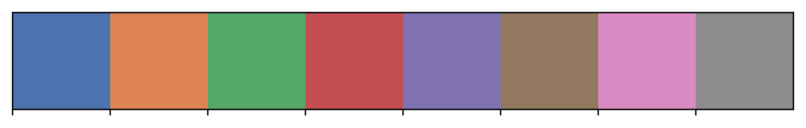
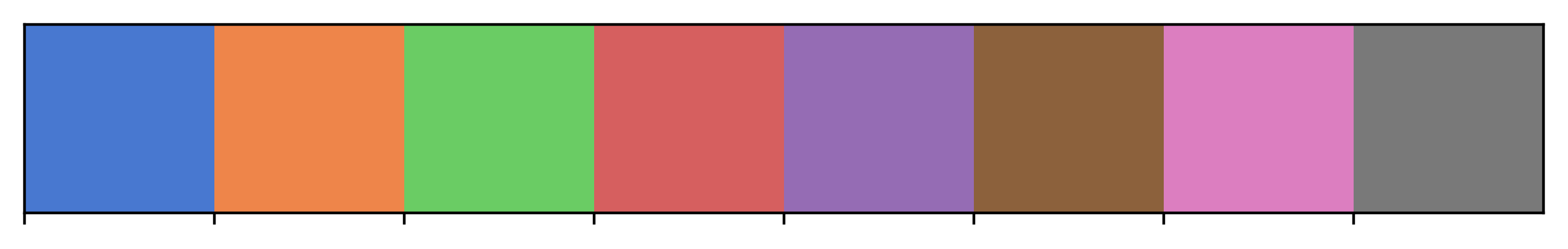
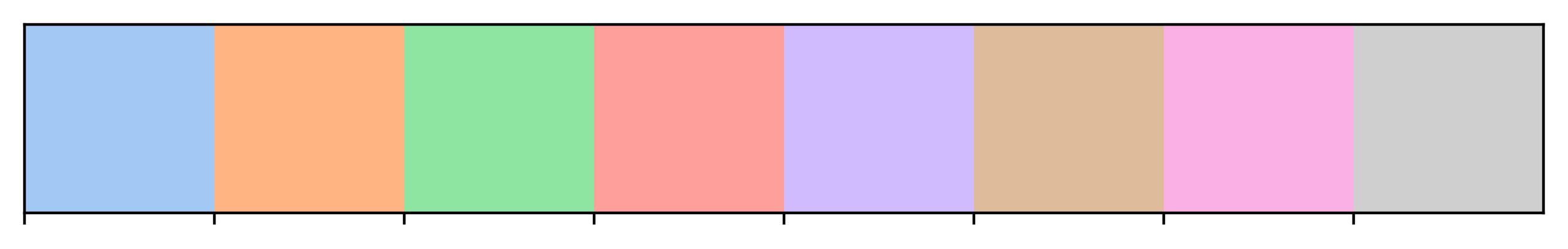
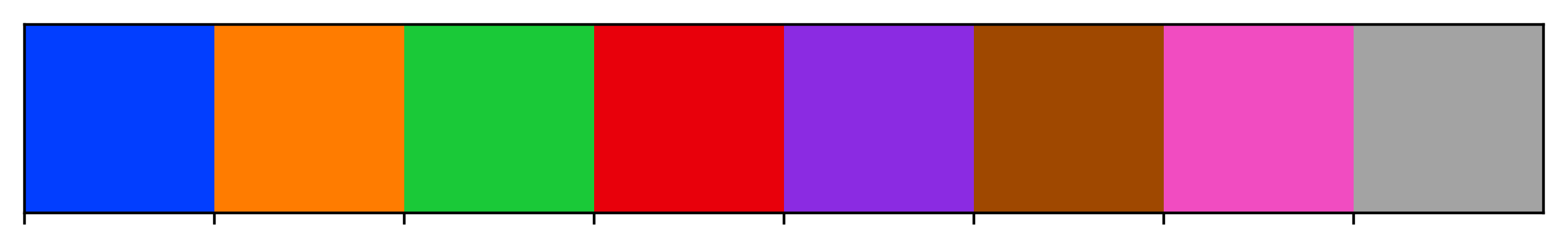
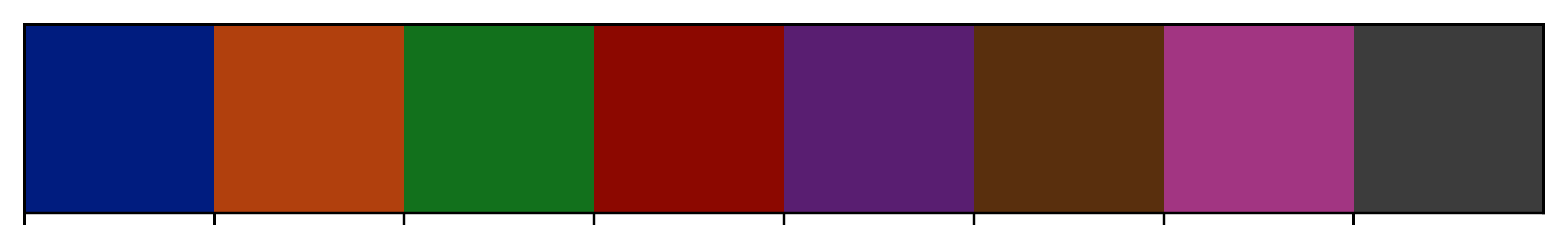
Seaborn provides carefully designed color palettes:

fig, axes = plt.subplots(3, 2, figsize=(16, 14))

palettes = ['deep', 'muted', 'pastel', 'bright', 'dark', 'colorblind']

for idx, palette in enumerate(palettes):
    row = idx // 2
    col = idx % 2
    
    colors = sns.color_palette(palette, 8)
    sns.palplot(colors, size=1)
    
    # Display in subplot
    axes[row, col].imshow([colors], aspect='auto')
    axes[row, col].set_title(f'Palette: {palette}', fontsize=16)
    axes[row, col].axis('off')

plt.tight_layout()
plt.show()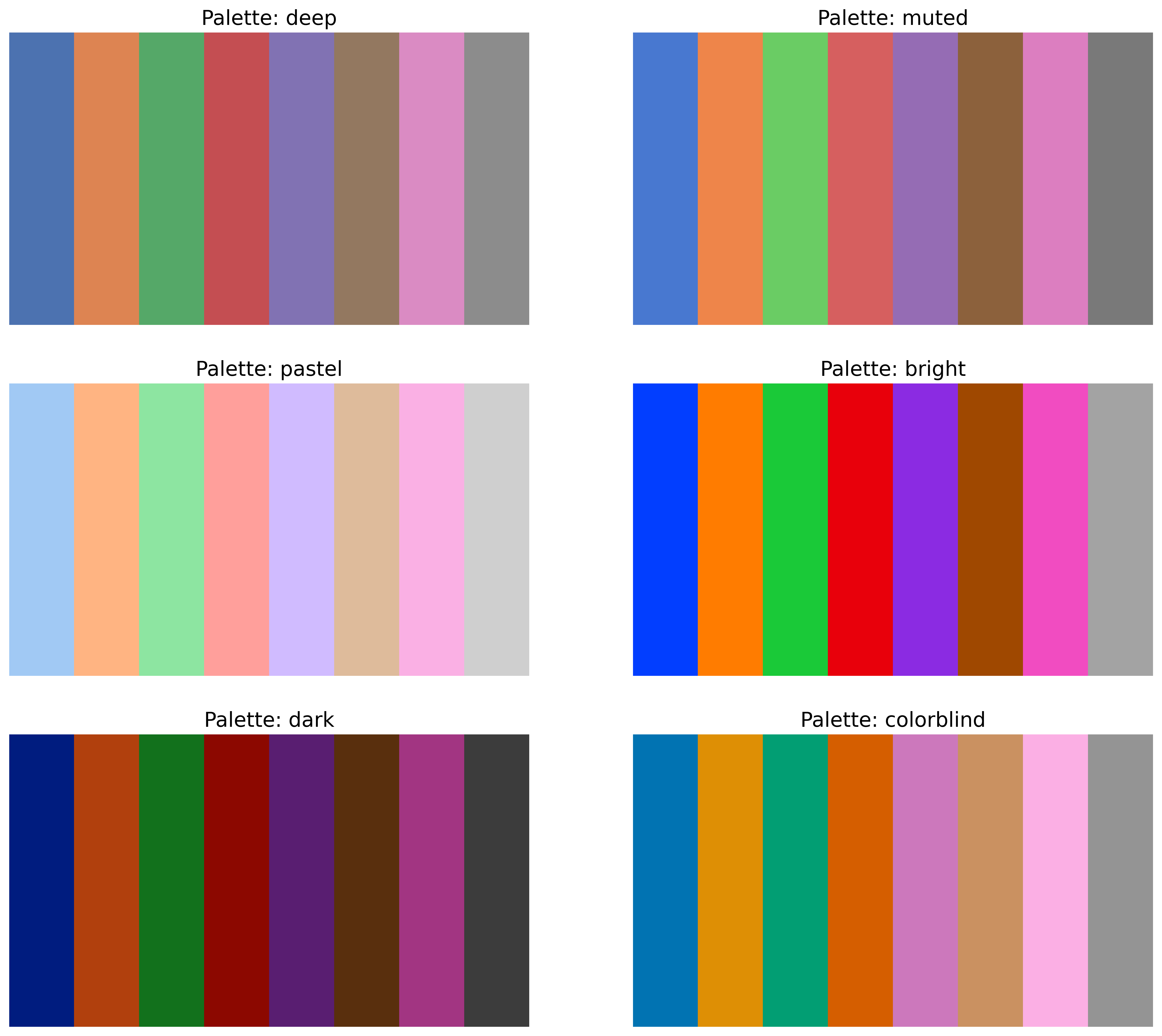

Use sns.set_palette() to apply a palette globally.

Scatter Plots with Hue

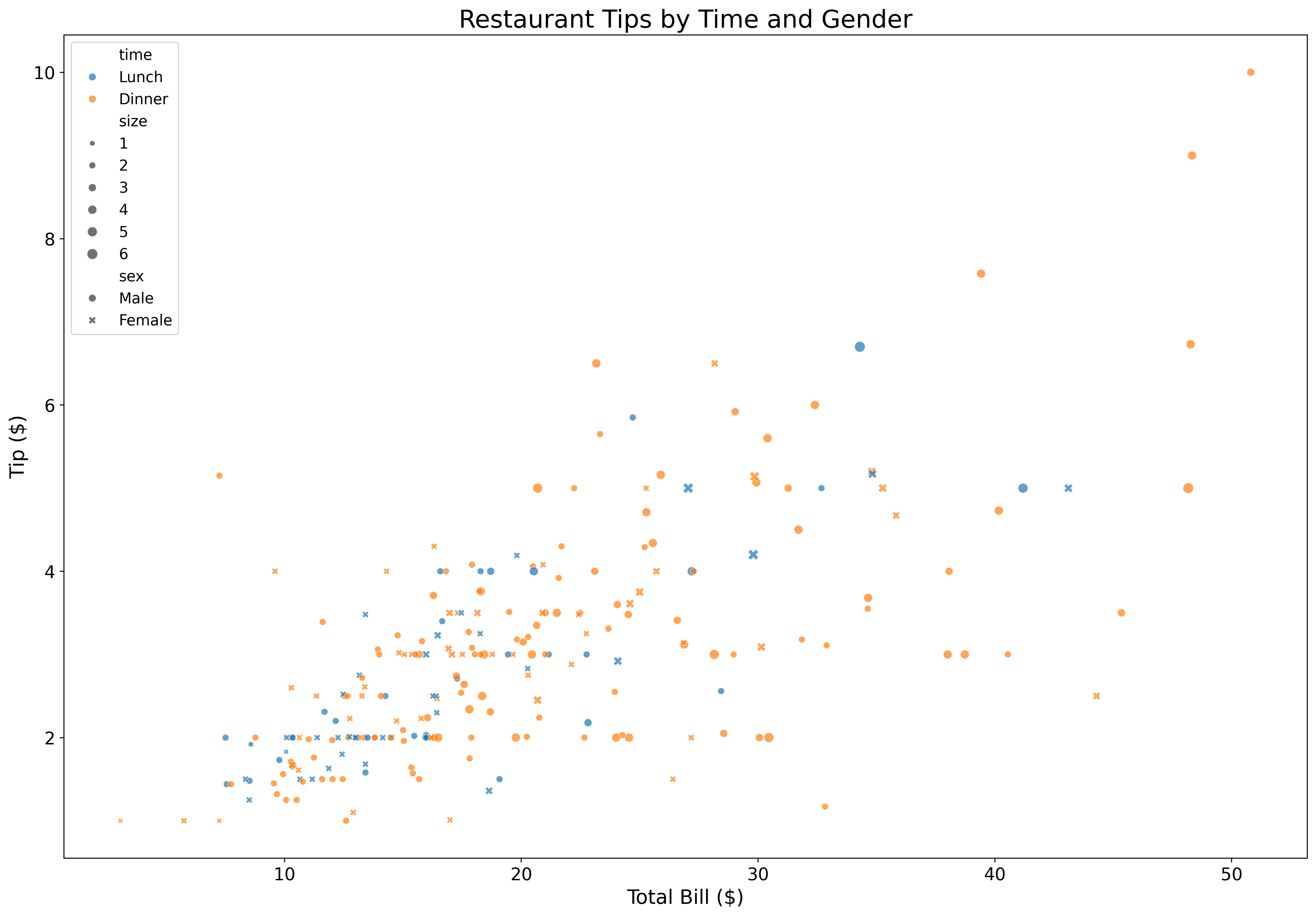
Add categorical dimensions with color:

fig, ax = plt.subplots(figsize=(18, 12))

tips = sns.load_dataset('tips')

sns.scatterplot(data=tips, 
                x='total_bill', 
                y='tip',
                hue='time',
                style='sex',
                size='size',
                alpha=0.7,
                ax=ax)

ax.set_xlabel('Total Bill ($)', fontsize=16)
ax.set_ylabel('Tip ($)', fontsize=16)
ax.set_title('Restaurant Tips by Time and Gender', fontsize=20)
ax.tick_params(labelsize=14)
ax.legend(fontsize=12)
plt.show()

Seaborn automatically creates beautiful legends for categorical variables.

Line Plots

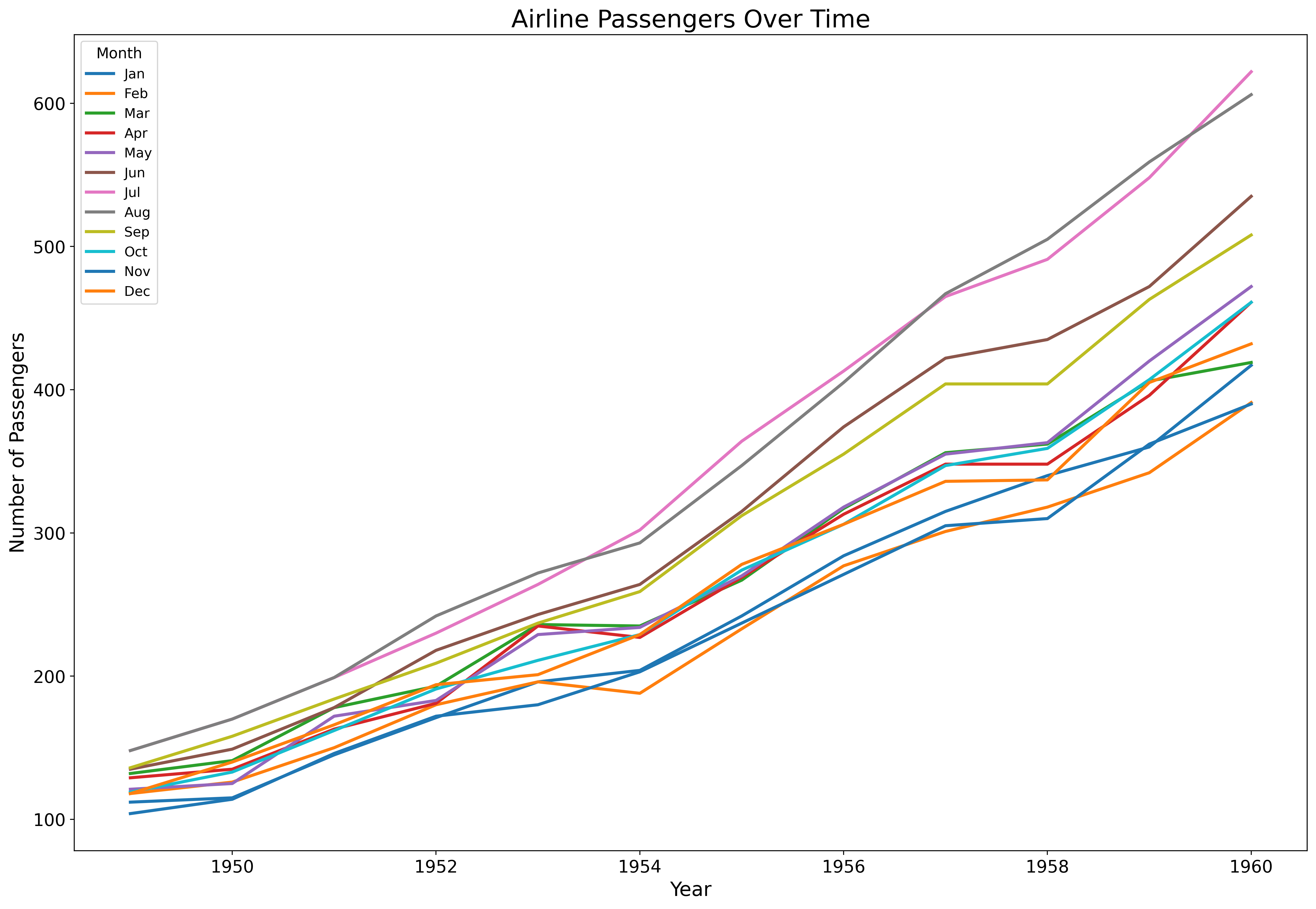
Perfect for time series and trends:

fig, ax = plt.subplots(figsize=(18, 12))

flights = sns.load_dataset('flights')

sns.lineplot(data=flights, 
             x='year', 
             y='passengers',
             hue='month',
             palette='tab10',
             linewidth=2.5,
             ax=ax)

ax.set_xlabel('Year', fontsize=16)
ax.set_ylabel('Number of Passengers', fontsize=16)
ax.set_title('Airline Passengers Over Time', fontsize=20)
ax.tick_params(labelsize=14)
ax.legend(title='Month', fontsize=11, title_fontsize=12)
plt.show()

Line plots automatically aggregate and show confidence intervals.

Bar Plots with Error Bars

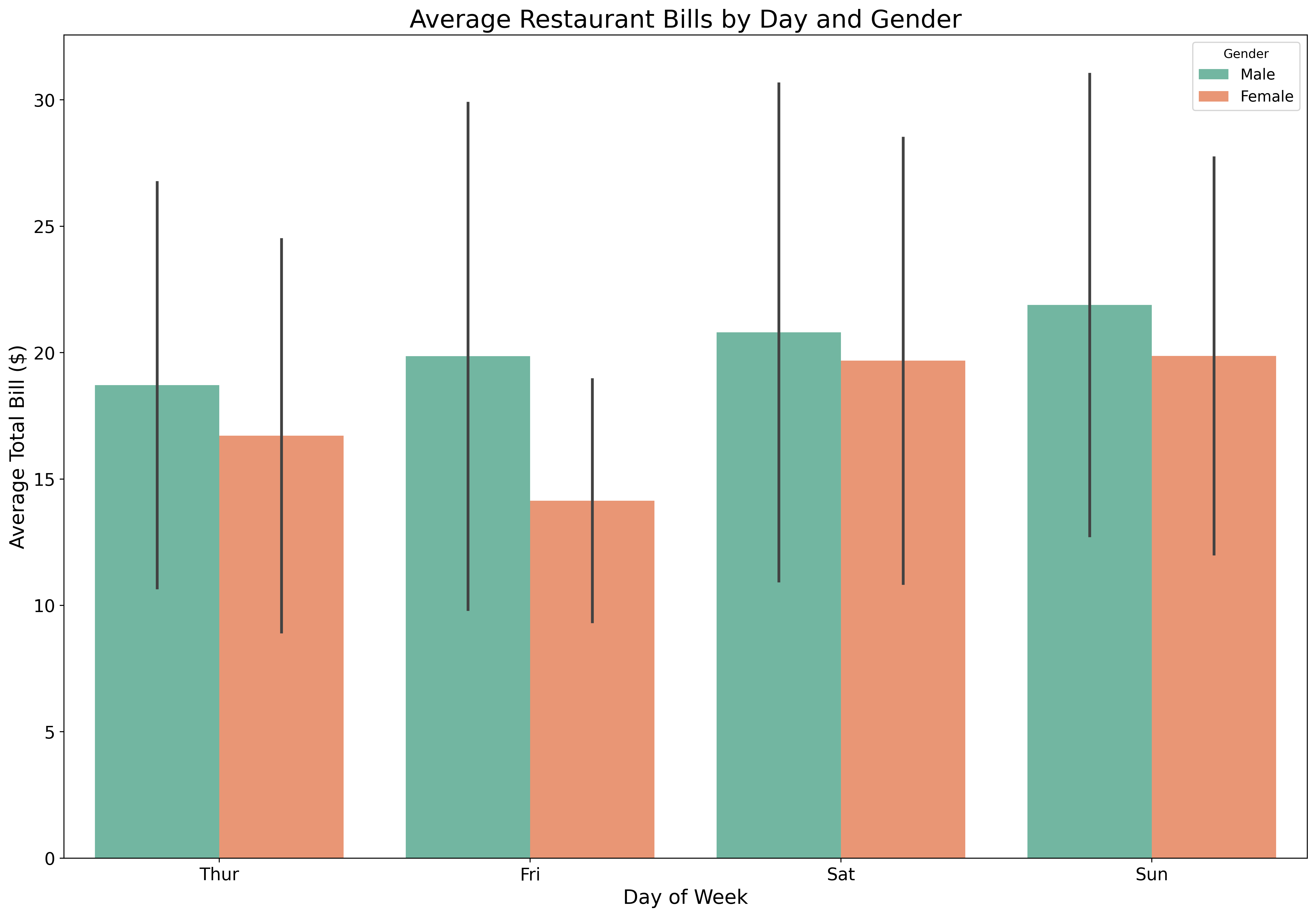
Show means and confidence intervals:

fig, ax = plt.subplots(figsize=(18, 12))

tips = sns.load_dataset('tips')

sns.barplot(data=tips,
            x='day',
            y='total_bill',
            hue='sex',
            palette='Set2',
            errorbar='sd',
            ax=ax)

ax.set_xlabel('Day of Week', fontsize=16)
ax.set_ylabel('Average Total Bill ($)', fontsize=16)
ax.set_title('Average Restaurant Bills by Day and Gender', fontsize=20)
ax.tick_params(labelsize=14)
ax.legend(title='Gender', fontsize=12)
plt.show()

Seaborn automatically calculates statistics and error bars!

Count Plots

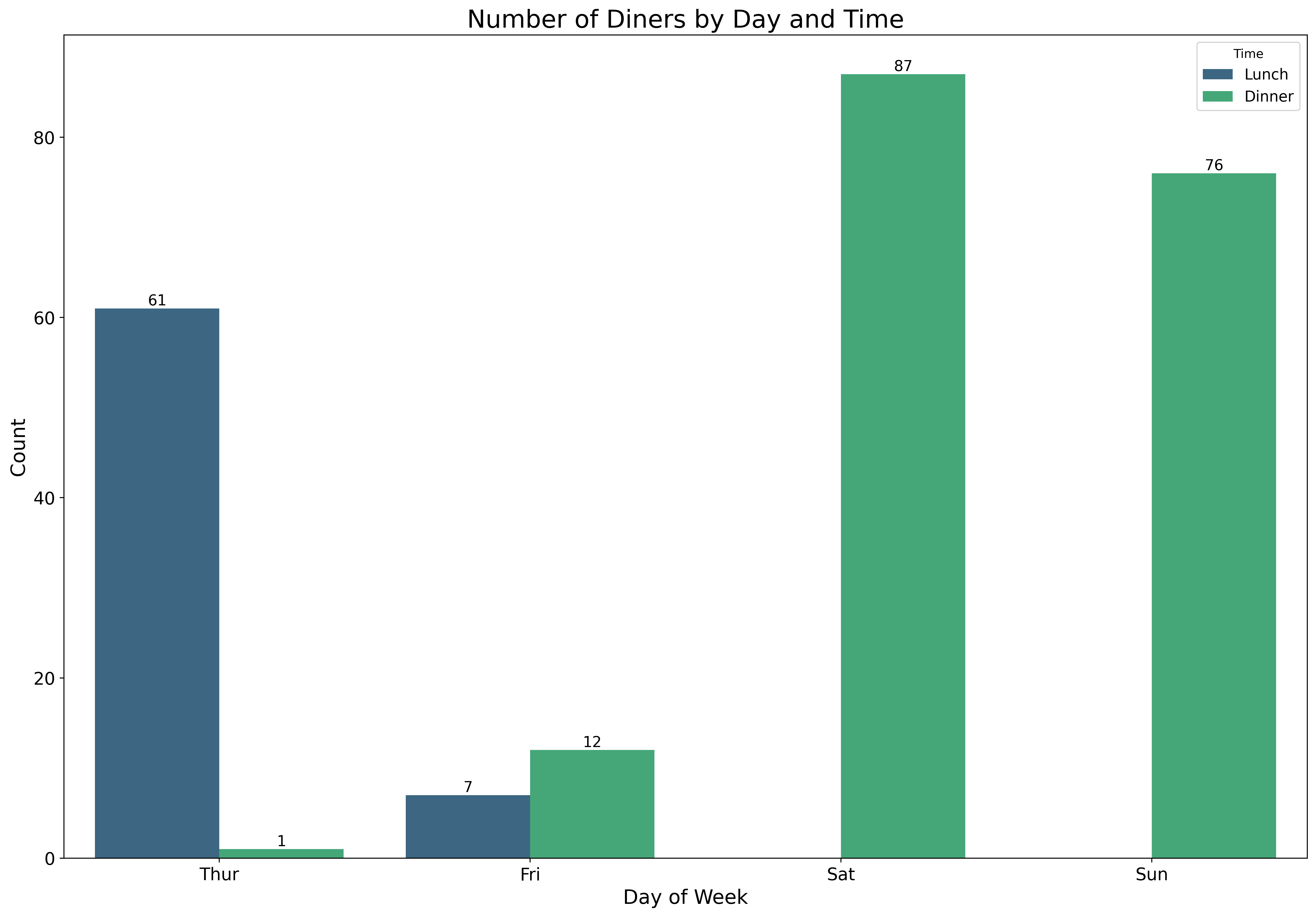
Visualize categorical distributions:

fig, ax = plt.subplots(figsize=(18, 12))

tips = sns.load_dataset('tips')

sns.countplot(data=tips,
              x='day',
              hue='time',
              palette='viridis',
              ax=ax)

ax.set_xlabel('Day of Week', fontsize=16)
ax.set_ylabel('Count', fontsize=16)
ax.set_title('Number of Diners by Day and Time', fontsize=20)
ax.tick_params(labelsize=14)
ax.legend(title='Time', fontsize=12)

# Add value labels on bars
for container in ax.containers:
    ax.bar_label(container, fontsize=12)

plt.show()

Count plots are perfect for showing frequencies of categorical variables.

Box Plots

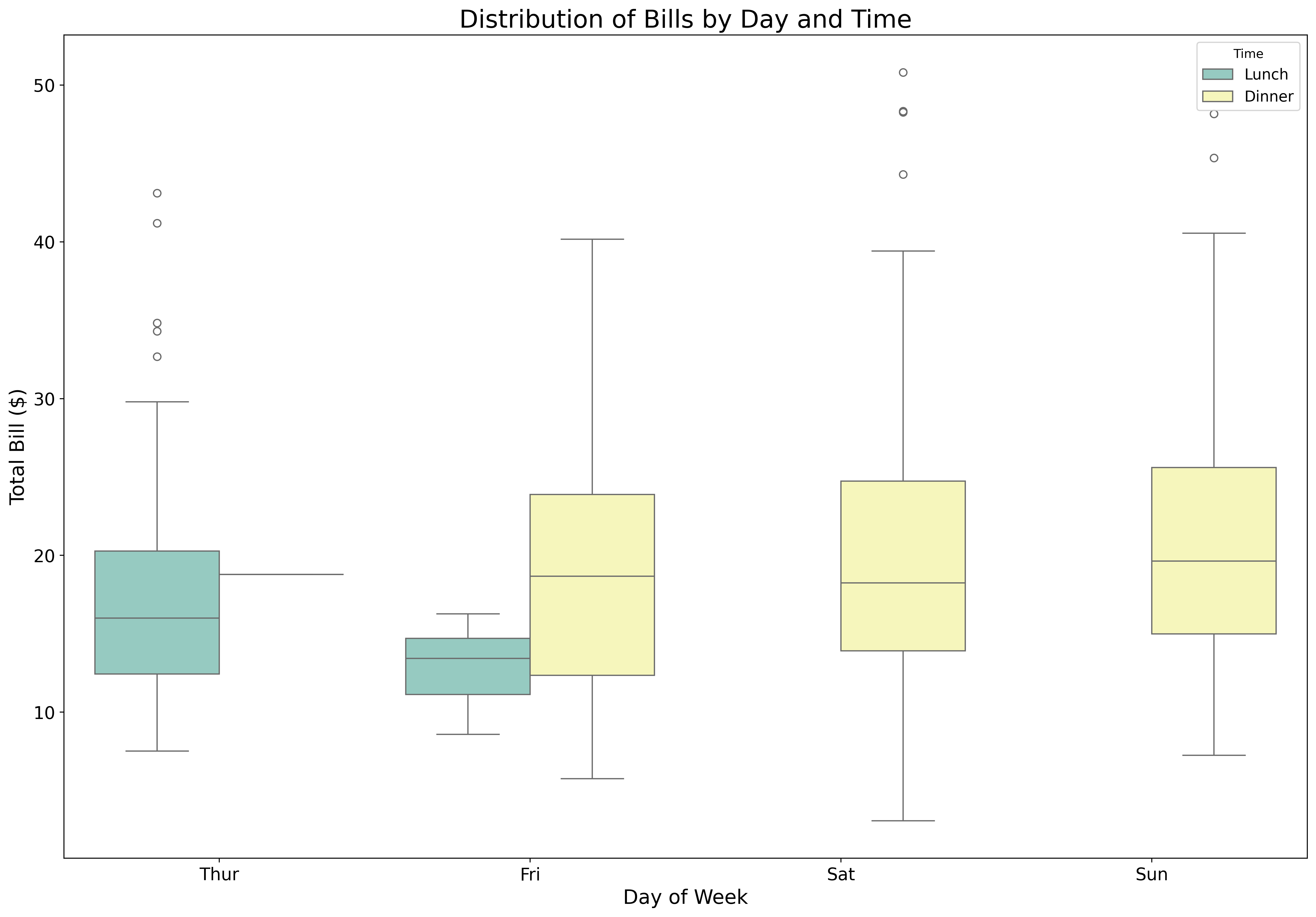
Display distributions with quartiles:

fig, ax = plt.subplots(figsize=(18, 12))

tips = sns.load_dataset('tips')

sns.boxplot(data=tips,
            x='day',
            y='total_bill',
            hue='time',
            palette='Set3',
            ax=ax)

ax.set_xlabel('Day of Week', fontsize=16)
ax.set_ylabel('Total Bill ($)', fontsize=16)
ax.set_title('Distribution of Bills by Day and Time', fontsize=20)
ax.tick_params(labelsize=14)
ax.legend(title='Time', fontsize=12)
plt.show()

Box plots show median, quartiles, and outliers - perfect for comparing distributions.

Violin Plots

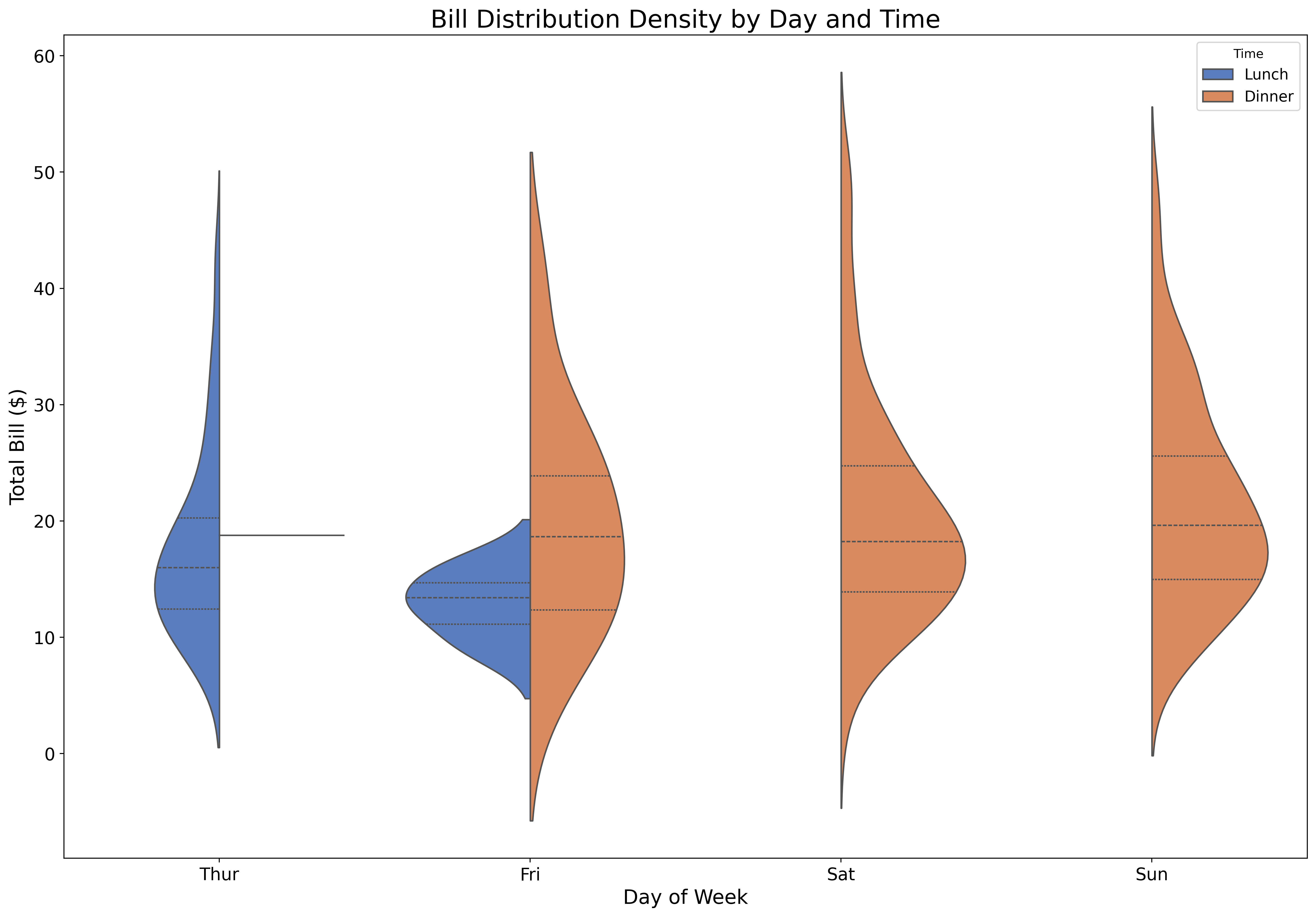
Combine box plots with distribution density:

fig, ax = plt.subplots(figsize=(18, 12))

tips = sns.load_dataset('tips')

sns.violinplot(data=tips,
               x='day',
               y='total_bill',
               hue='time',
               split=True,
               palette='muted',
               inner='quartile',
               ax=ax)

ax.set_xlabel('Day of Week', fontsize=16)
ax.set_ylabel('Total Bill ($)', fontsize=16)
ax.set_title('Bill Distribution Density by Day and Time', fontsize=20)
ax.tick_params(labelsize=14)
ax.legend(title='Time', fontsize=12)
plt.show()

Violin plots reveal the full distribution shape, showing where data is concentrated.

Strip and Swarm Plots

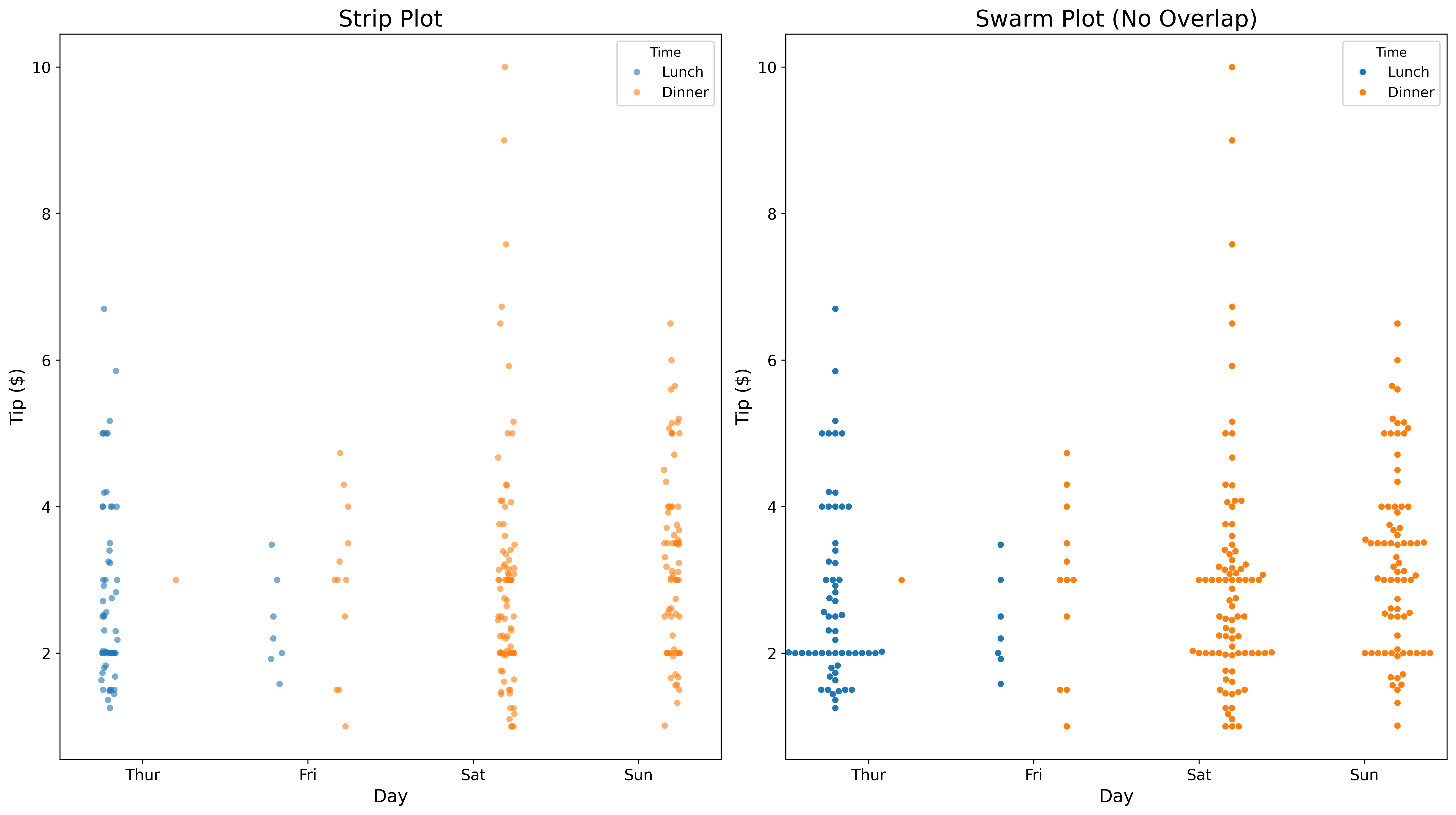
Show individual data points:

fig, axes = plt.subplots(1, 2, figsize=(16, 9))

tips = sns.load_dataset('tips')

# Strip plot
sns.stripplot(data=tips,
              x='day',
              y='tip',
              hue='time',
              dodge=True,
              alpha=0.6,
              ax=axes[0])
axes[0].set_title('Strip Plot', fontsize=18)
axes[0].set_xlabel('Day', fontsize=14)
axes[0].set_ylabel('Tip ($)', fontsize=14)
axes[0].tick_params(labelsize=12)
axes[0].legend(title='Time', fontsize=11)

# Swarm plot
sns.swarmplot(data=tips,
              x='day',
              y='tip',
              hue='time',
              dodge=True,
              ax=axes[1])
axes[1].set_title('Swarm Plot (No Overlap)', fontsize=18)
axes[1].set_xlabel('Day', fontsize=14)
axes[1].set_ylabel('Tip ($)', fontsize=14)
axes[1].tick_params(labelsize=12)
axes[1].legend(title='Time', fontsize=11)

plt.tight_layout()
plt.show()

Strip plots show all points; swarm plots arrange them to avoid overlap.

Histograms with KDE

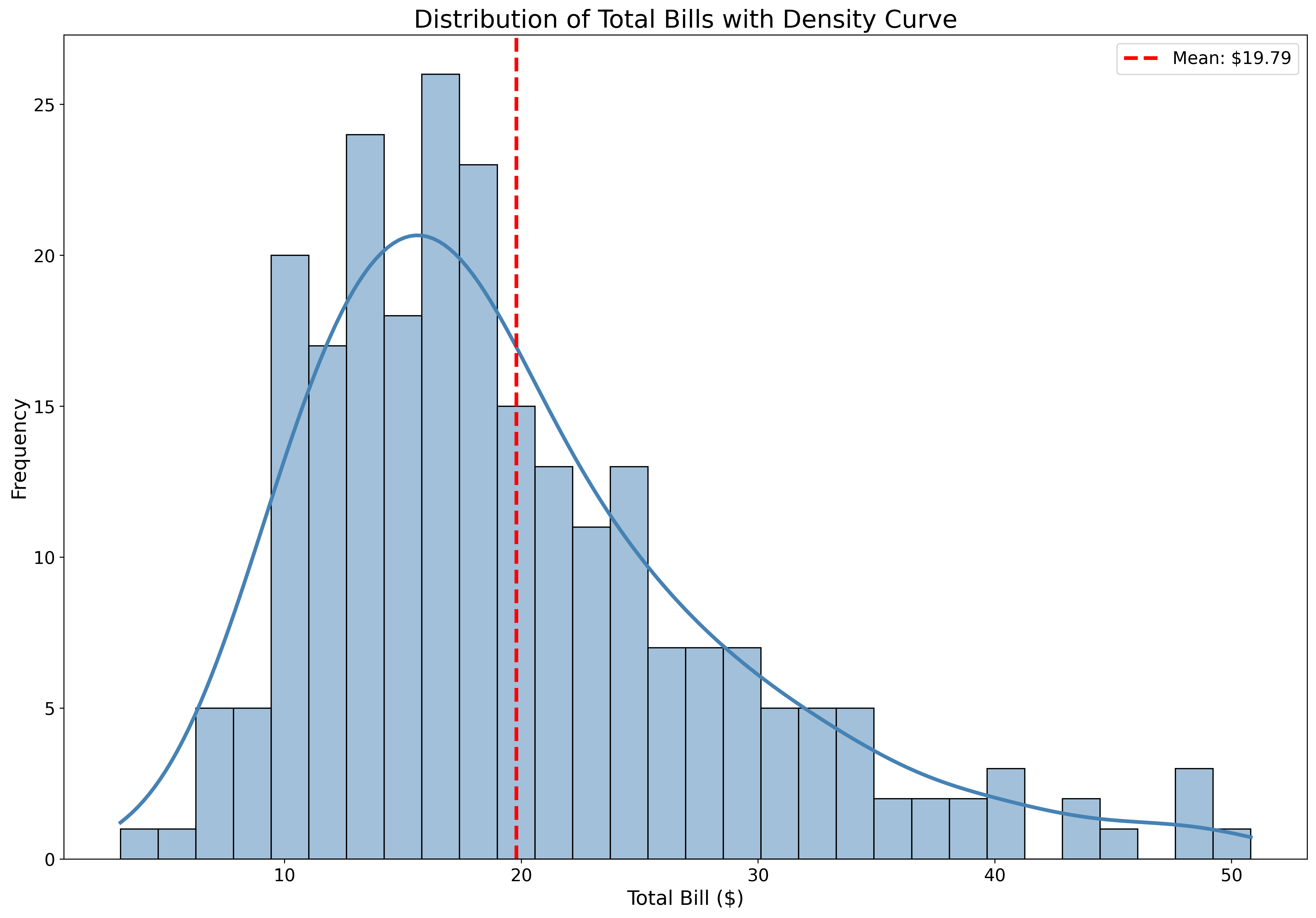
Combine histograms with density curves:

fig, ax = plt.subplots(figsize=(18, 12))

tips = sns.load_dataset('tips')

sns.histplot(data=tips,
             x='total_bill',
             kde=True,
             color='steelblue',
             bins=30,
             line_kws={'linewidth': 3},
             ax=ax)

ax.set_xlabel('Total Bill ($)', fontsize=16)
ax.set_ylabel('Frequency', fontsize=16)
ax.set_title('Distribution of Total Bills with Density Curve', fontsize=20)
ax.tick_params(labelsize=14)
ax.axvline(tips['total_bill'].mean(), color='red', linestyle='--', 
           linewidth=3, label=f'Mean: ${tips["total_bill"].mean():.2f}')
ax.legend(fontsize=14)
plt.show()

KDE (Kernel Density Estimation) shows the smooth distribution shape.

Overlapping Distributions

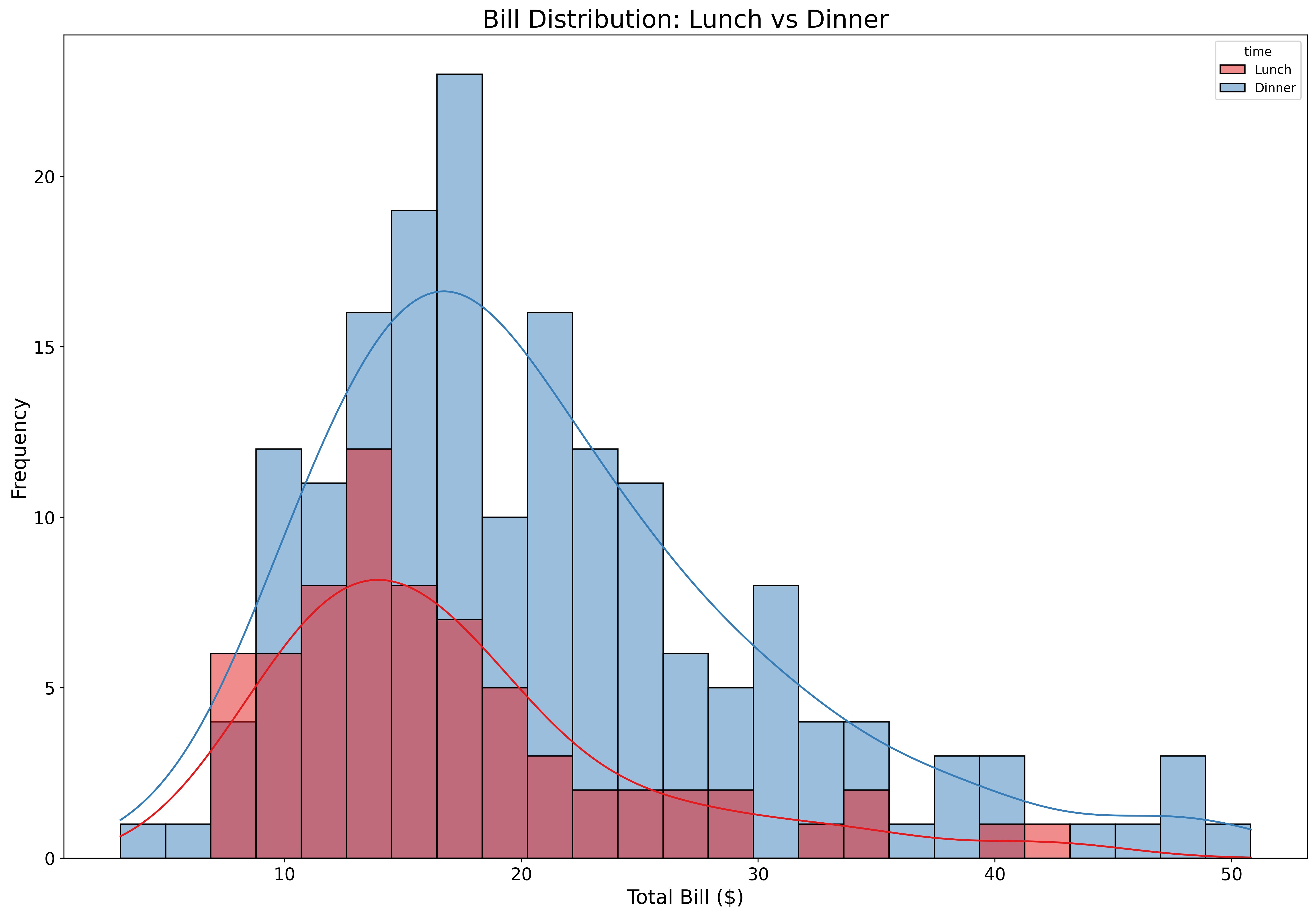
Compare multiple distributions:

fig, ax = plt.subplots(figsize=(18, 12))

tips = sns.load_dataset('tips')

sns.histplot(data=tips,
             x='total_bill',
             hue='time',
             kde=True,
             alpha=0.5,
             bins=25,
             palette='Set1',
             legend = True,
             ax=ax)

ax.set_xlabel('Total Bill ($)', fontsize=16)
ax.set_ylabel('Frequency', fontsize=16)
ax.set_title('Bill Distribution: Lunch vs Dinner', fontsize=20)
ax.tick_params(labelsize=14)
plt.show()

Overlapping histograms reveal differences in distributions between groups.

KDE Plots

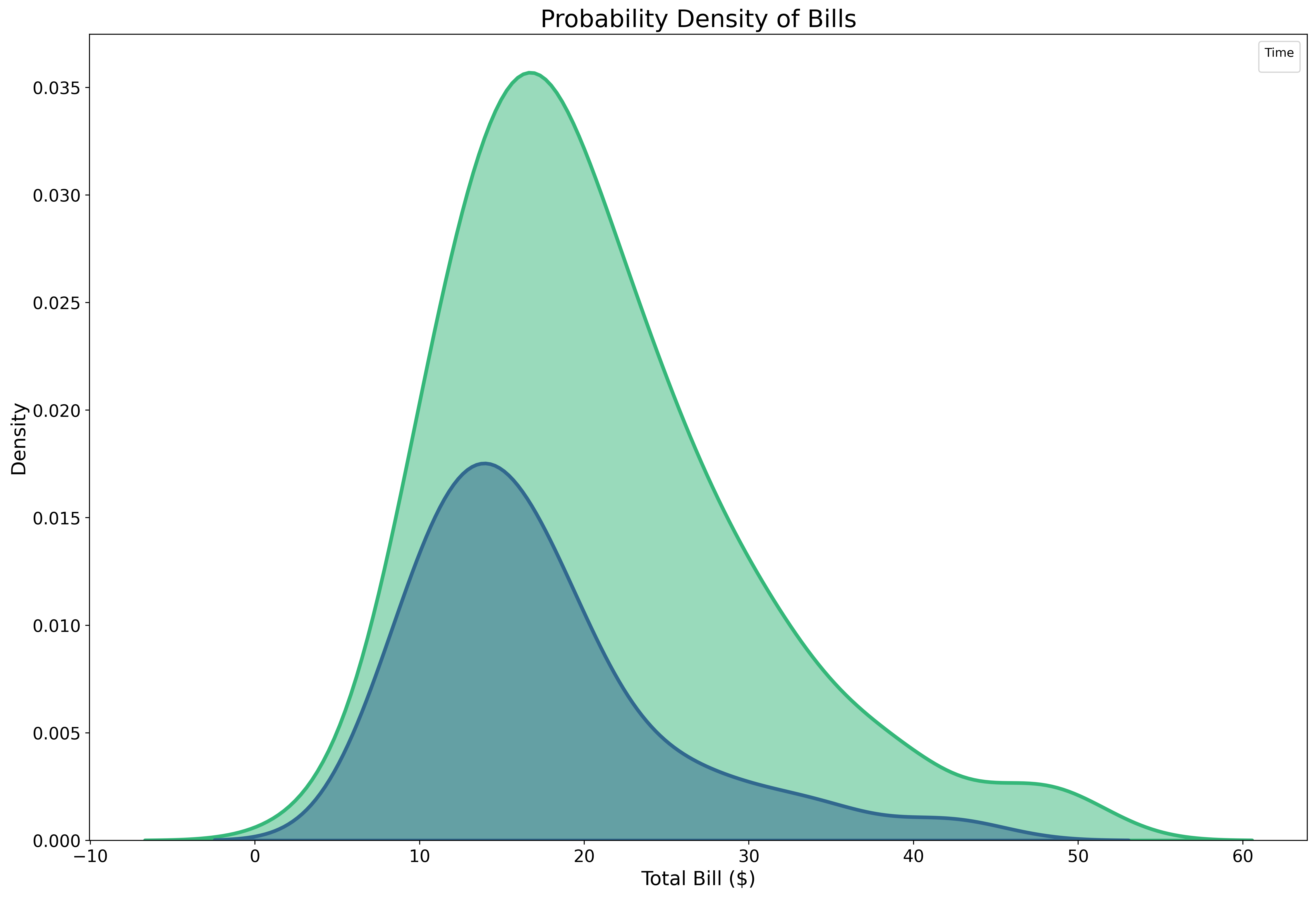
Pure density visualization:

fig, ax = plt.subplots(figsize=(18, 12))

tips = sns.load_dataset('tips')

sns.kdeplot(data=tips,
            x='total_bill',
            hue='time',
            fill=True,
            alpha=0.5,
            linewidth=3,
            palette='viridis',
            ax=ax)

ax.set_xlabel('Total Bill ($)', fontsize=16)
ax.set_ylabel('Density', fontsize=16)
ax.set_title('Probability Density of Bills', fontsize=20)
ax.tick_params(labelsize=14)
ax.legend(title='Time', fontsize=12)
plt.show()

KDE plots are smooth, continuous representations of distributions.

Regression Plots

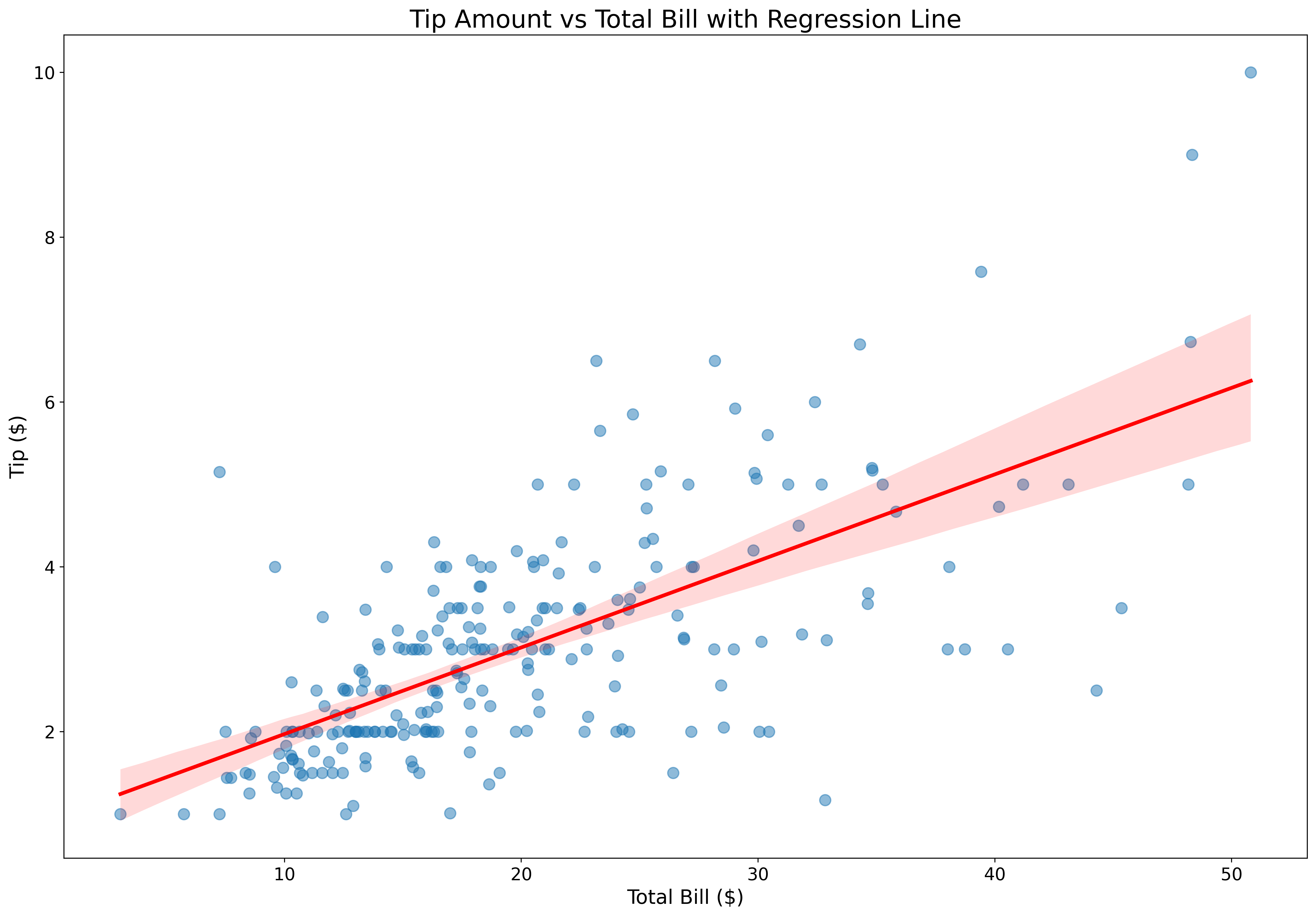
Add trend lines effortlessly:

fig, ax = plt.subplots(figsize=(18, 12))

tips = sns.load_dataset('tips')

sns.regplot(data=tips,
            x='total_bill',
            y='tip',
            scatter_kws={'alpha': 0.5, 's': 80},
            line_kws={'color': 'red', 'linewidth': 3},
            ax=ax)

ax.set_xlabel('Total Bill ($)', fontsize=16)
ax.set_ylabel('Tip ($)', fontsize=16)
ax.set_title('Tip Amount vs Total Bill with Regression Line', fontsize=20)
ax.tick_params(labelsize=14)
plt.show()

Regression plots automatically fit and display trend lines with confidence intervals.

Multiple Regressions

Compare relationships across categories:

fig, ax = plt.subplots(figsize=(18, 12))

tips = sns.load_dataset('tips')

sns.lmplot(data=tips,
           x='total_bill',
           y='tip',
           hue='smoker',
           height=9,
           aspect=14/9,
           scatter_kws={'alpha': 0.5, 's': 80},
           line_kws={'linewidth': 3},
           palette='Set1')

plt.xlabel('Total Bill ($)', fontsize=16)
plt.ylabel('Tip ($)', fontsize=16)
plt.title('Tip Patterns: Smokers vs Non-Smokers', fontsize=20)
plt.tick_params(labelsize=14)
plt.legend(title='Smoker', fontsize=12)
plt.show()

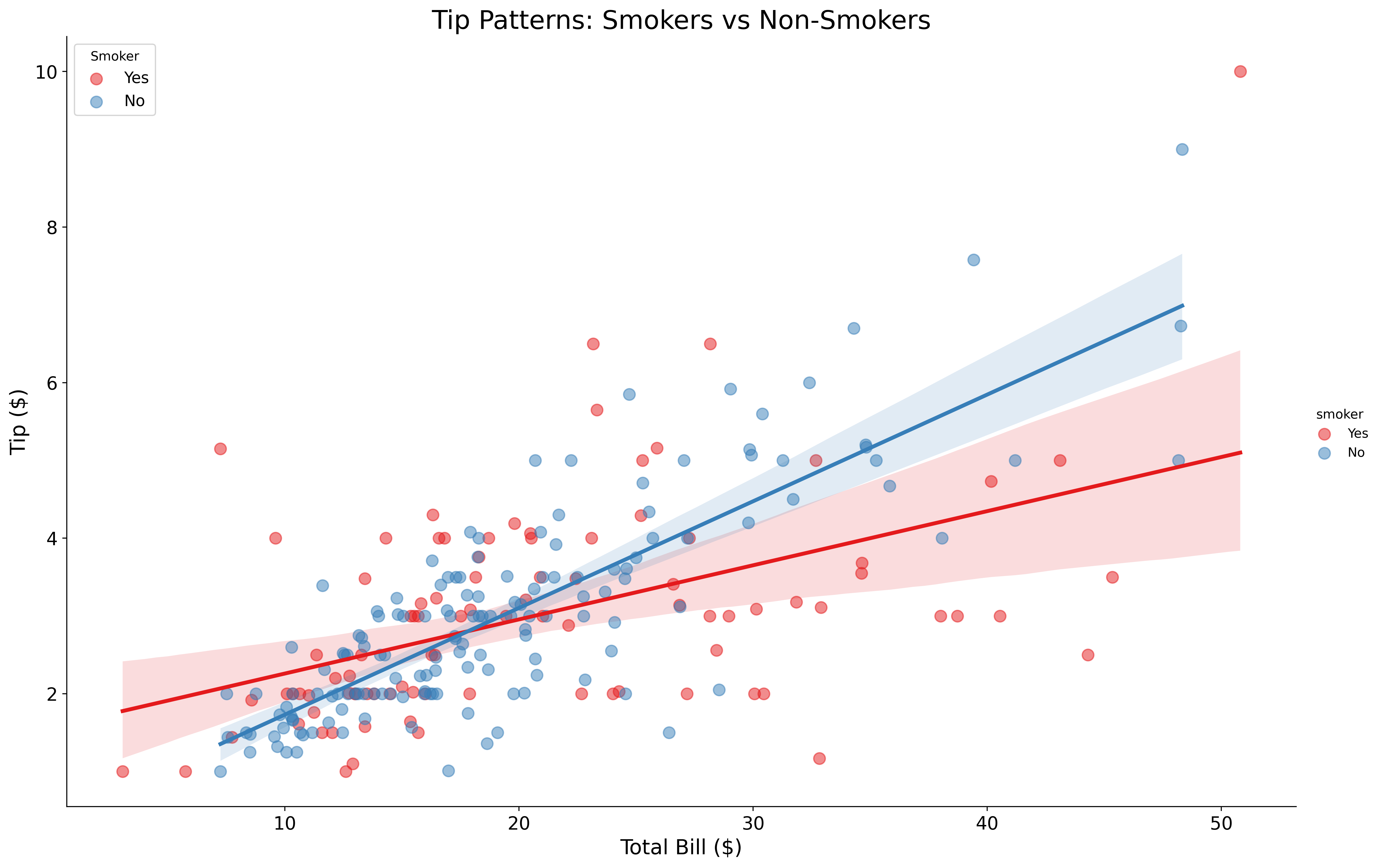
lmplot creates separate regression lines for each category.

Residual Plots

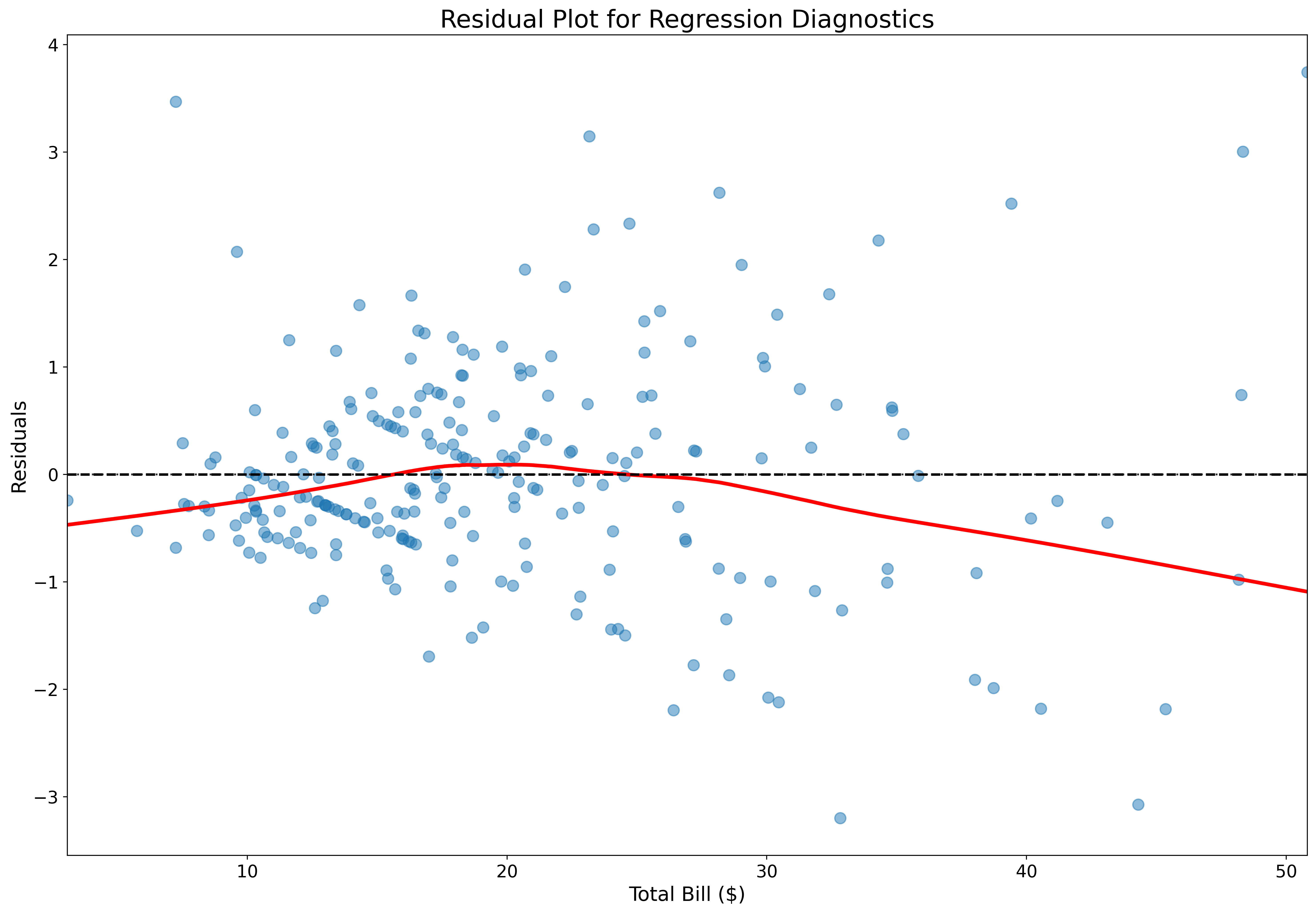
Assess regression quality:

fig, ax = plt.subplots(figsize=(18, 12))

tips = sns.load_dataset('tips')

sns.residplot(data=tips,
              x='total_bill',
              y='tip',
              lowess=True,
              scatter_kws={'alpha': 0.5, 's': 80},
              line_kws={'color': 'red', 'linewidth': 3},
              ax=ax)

ax.set_xlabel('Total Bill ($)', fontsize=16)
ax.set_ylabel('Residuals', fontsize=16)
ax.set_title('Residual Plot for Regression Diagnostics', fontsize=20)
ax.tick_params(labelsize=14)
ax.axhline(0, color='black', linestyle='--', linewidth=2)
plt.show()

Residual plots help identify non-linear patterns and heteroscedasticity.

Heatmaps with Annotations

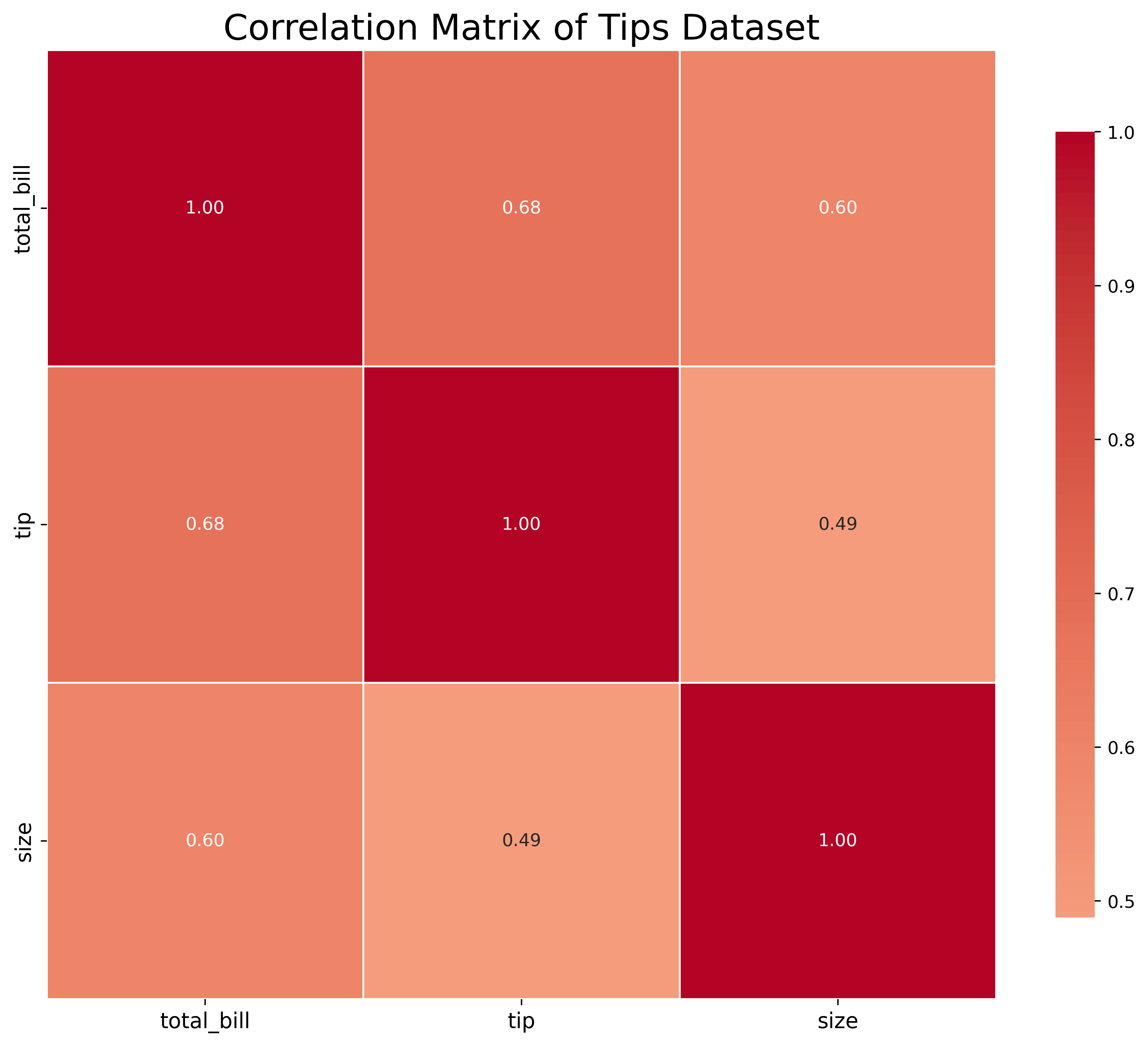
Visualize correlation matrices:

fig, ax = plt.subplots(figsize=(12, 10))

tips = sns.load_dataset('tips')
numeric_cols = tips.select_dtypes(include=[np.number])
correlation = numeric_cols.corr()

sns.heatmap(correlation,
            annot=True,
            fmt='.2f',
            cmap='coolwarm',
            center=0,
            square=True,
            linewidths=1,
            cbar_kws={'shrink': 0.8},
            ax=ax)

ax.set_title('Correlation Matrix of Tips Dataset', fontsize=20)
ax.tick_params(labelsize=12)
plt.show()

Heatmaps make correlation patterns immediately visible.

Pair Plots

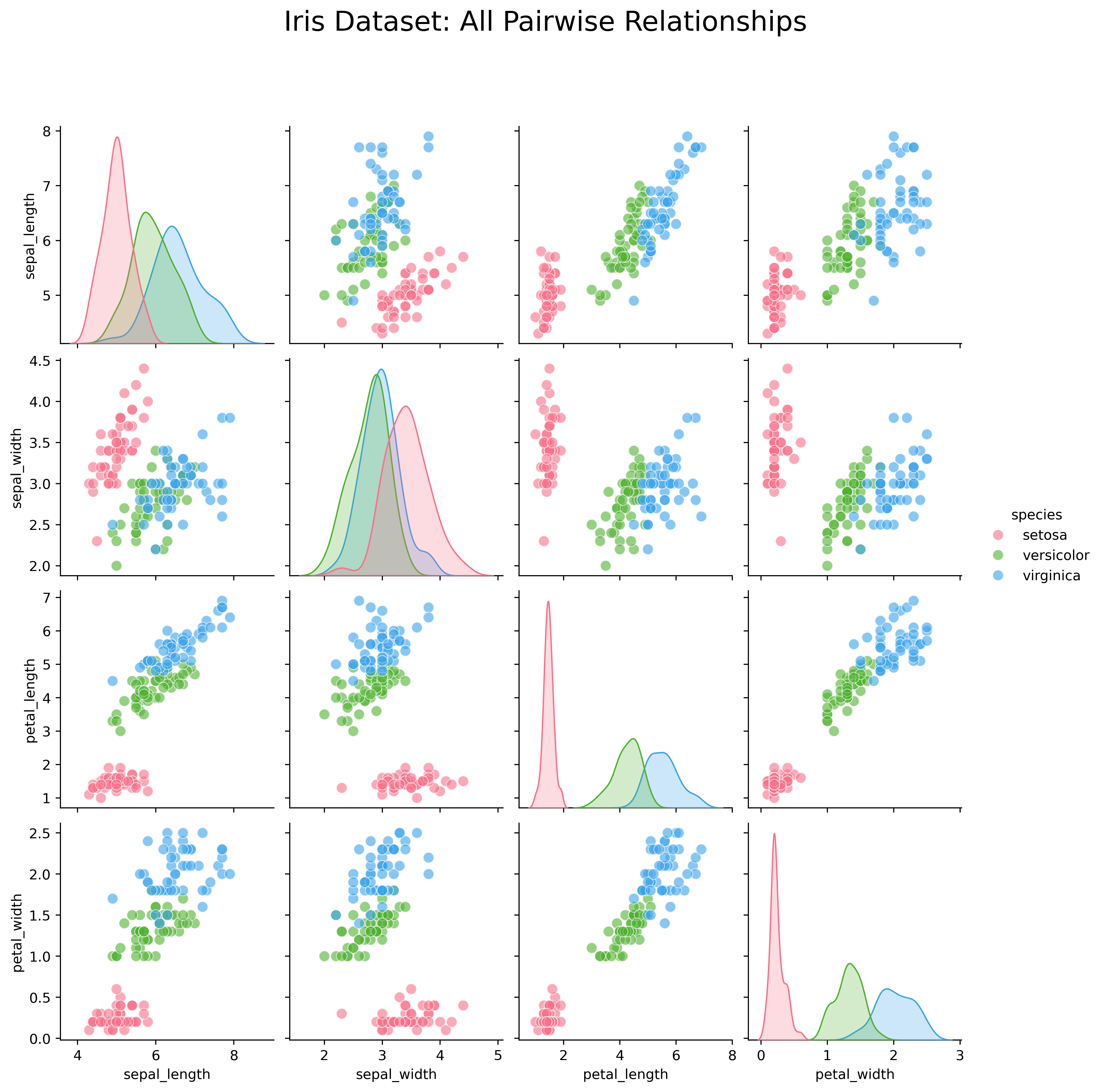
Explore all pairwise relationships:

iris = sns.load_dataset('iris')

g = sns.pairplot(iris,
                 hue='species',
                 palette='husl',
                 height=2.5,
                 aspect=1,
                 diag_kind='kde',
                 plot_kws={'alpha': 0.6, 's': 60})

g.fig.suptitle('Iris Dataset: All Pairwise Relationships', 
               fontsize=20, y=1.1)
plt.show()

Pair plots are invaluable for exploratory data analysis and feature selection.

Joint Plots

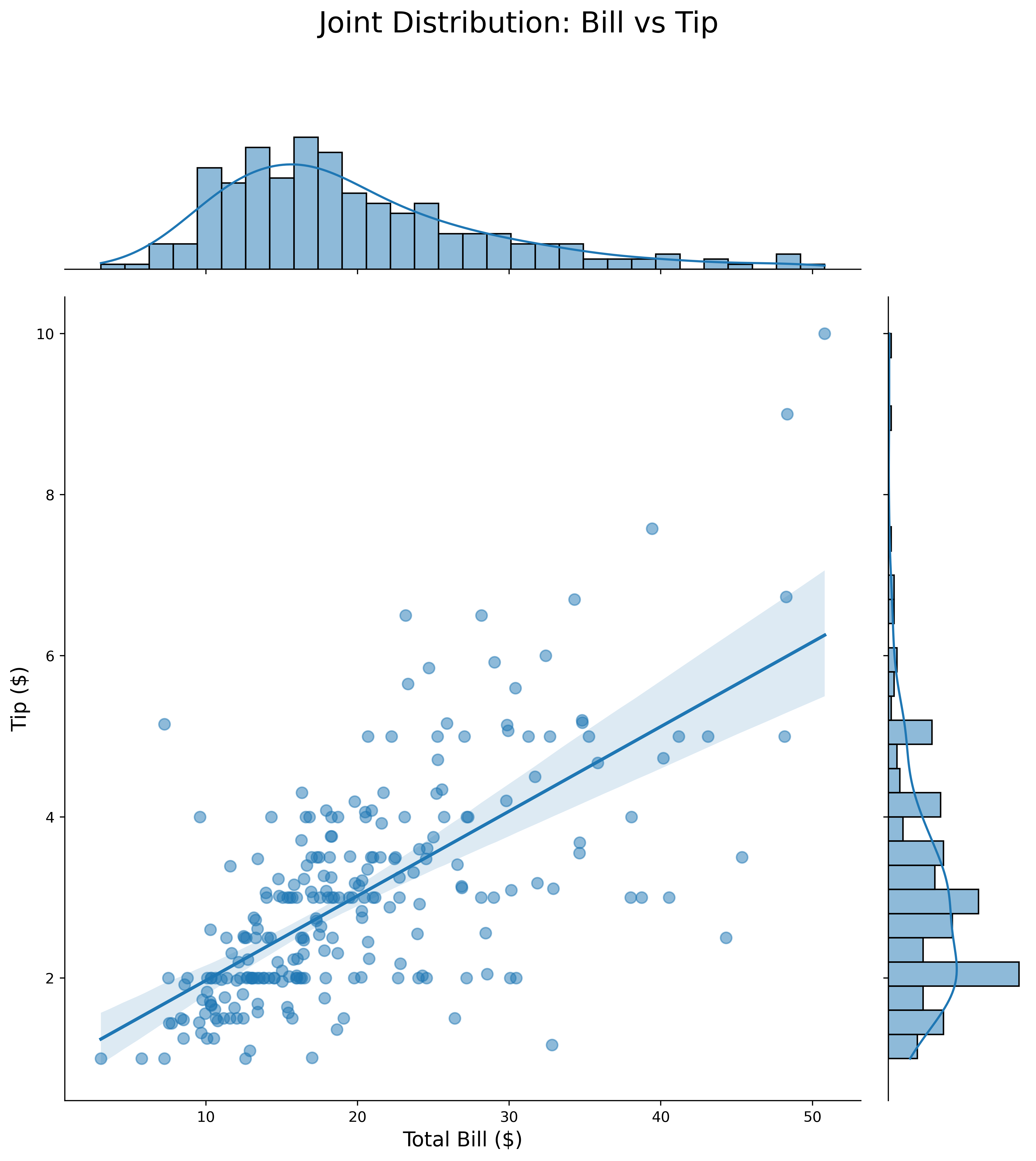
Combine scatter with marginal distributions:

tips = sns.load_dataset('tips')

g = sns.jointplot(data=tips,
                  x='total_bill',
                  y='tip',
                  kind='reg',
                  height=10,
                  ratio=5,
                  marginal_kws={'bins': 30, 'kde': True},
                  joint_kws={'scatter_kws': {'alpha': 0.5, 's': 60}})

g.fig.suptitle('Joint Distribution: Bill vs Tip', fontsize=20, y=1.1)
g.set_axis_labels('Total Bill ($)', 'Tip ($)', fontsize=14)
plt.show()

Joint plots show both the relationship and individual distributions simultaneously.

FacetGrid: Small Multiples

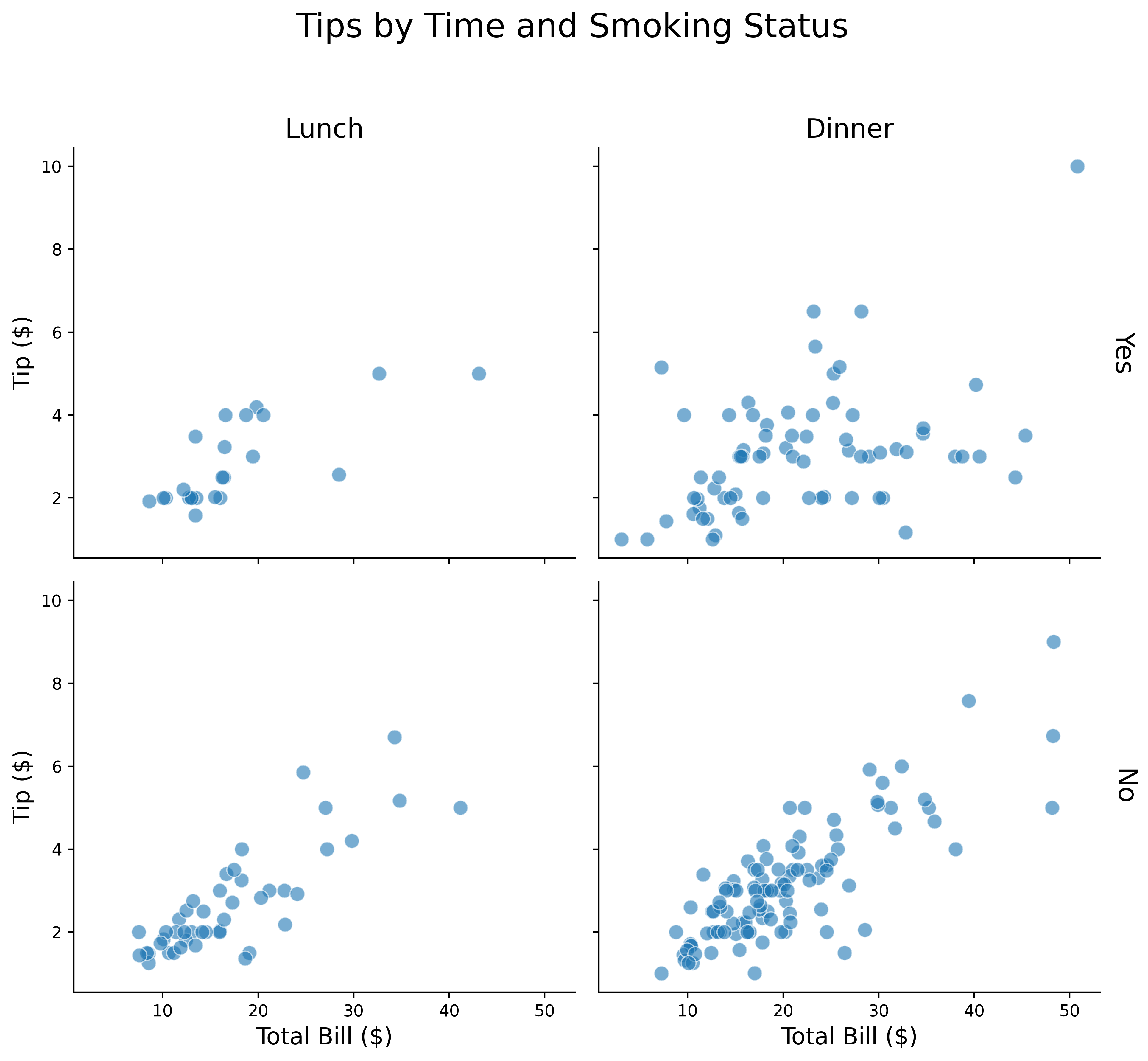
Create grids of plots by category:

tips = sns.load_dataset('tips')

g = sns.FacetGrid(tips, 
                  col='time', 
                  row='smoker',
                  height=4, 
                  aspect=1.2,
                  margin_titles=True)

g.map_dataframe(sns.scatterplot, 
                x='total_bill', 
                y='tip',
                alpha=0.6,
                s=80)

g.set_axis_labels('Total Bill ($)', 'Tip ($)', fontsize=14)
g.set_titles(col_template='{col_name}', row_template='{row_name}', size=16)
g.fig.suptitle('Tips by Time and Smoking Status', fontsize=20, y=1.1)
plt.show()

FacetGrid is perfect for comparing subgroups side-by-side.

Custom FacetGrid Functions

Apply any plot function to grid:

tips = sns.load_dataset('tips')

g = sns.FacetGrid(tips,
                  col='day',
                  col_wrap=2,
                  height=4.5,
                  aspect=1.2)

g.map_dataframe(sns.histplot,
                x='total_bill',
                kde=True,
                bins=20,
                color='steelblue')

g.set_axis_labels('Total Bill ($)', 'Count', fontsize=14)
g.set_titles(col_template='Day: {col_name}', size=16)
g.fig.suptitle('Bill Distributions by Day of Week', fontsize=20, y=1.1)
plt.show()

Use col_wrap to control the grid layout.

Categorical Plots with catplot

Unified interface for categorical data:

tips = sns.load_dataset('tips')

g = sns.catplot(data=tips,
                x='day',
                y='total_bill',
                hue='sex',
                col='time',
                kind='box',
                height=5,
                aspect=1.2,
                palette='Set2')

g.set_axis_labels('Day of Week', 'Total Bill ($)', fontsize=14)
g.set_titles(col_template='Time: {col_name}', size=16)
g.fig.suptitle('Bills by Day, Gender, and Time', fontsize=20, y=1.1)
plt.show()

catplot provides a consistent interface for all categorical plots.

Relational Plots with relplot

Unified interface for relational data:

tips = sns.load_dataset('tips')

g = sns.relplot(data=tips,
                x='total_bill',
                y='tip',
                hue='smoker',
                size='size',
                col='time',
                row='sex',
                kind='scatter',
                height=4,
                aspect=1.2,
                sizes=(50, 300),
                alpha=0.7,
                palette='viridis')

g.set_axis_labels('Total Bill ($)', 'Tip ($)', fontsize=12)
g.set_titles(col_template='{col_name}', row_template='{row_name}', size=14)
g.fig.suptitle('Comprehensive Tip Analysis', fontsize=18, y=1.1)
plt.show()

relplot handles scatter and line plots with faceting.

Distribution Plots: displot

Comprehensive distribution visualization:

tips = sns.load_dataset('tips')

g = sns.displot(data=tips,
                x='total_bill',
                hue='time',
                col='day',
                kind='kde',
                fill=True,
                height=4,
                aspect=1.2,
                palette='muted')

g.set_axis_labels('Total Bill ($)', 'Density', fontsize=14)
g.set_titles(col_template='Day: {col_name}', size=16)
g.fig.suptitle('Bill Distributions Across Days', fontsize=20, y=1.1)
plt.show()

displot combines histograms, KDE, and ECDF with faceting.

Rug Plots

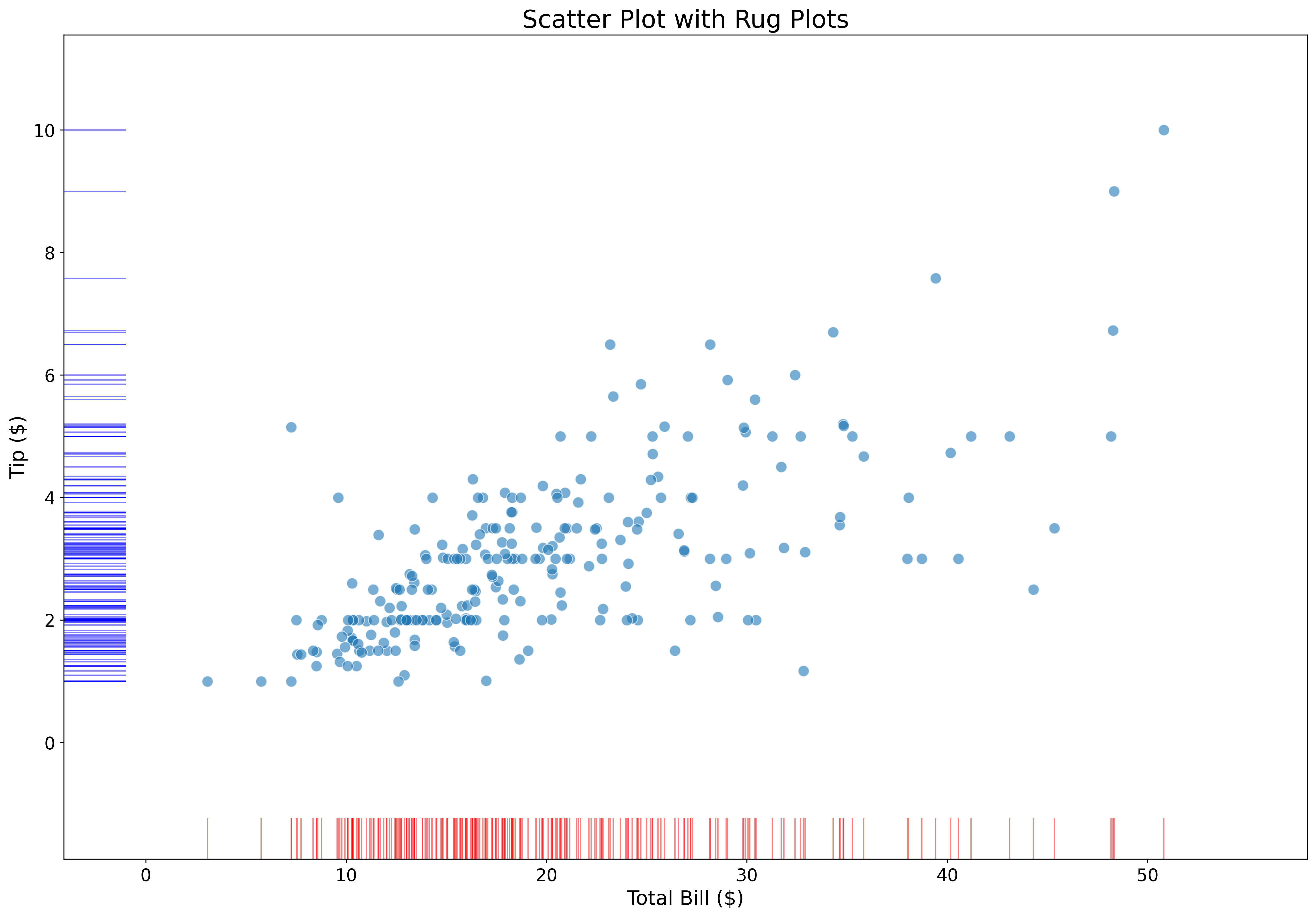
Add marginal tick marks:

fig, ax = plt.subplots(figsize=(18, 12))

tips = sns.load_dataset('tips')

sns.scatterplot(data=tips,
                x='total_bill',
                y='tip',
                alpha=0.6,
                s=80,
                ax=ax)

sns.rugplot(data=tips,
            x='total_bill',
            height=0.05,
            color='red',
            alpha=0.5,
            ax=ax)

sns.rugplot(data=tips,
            y='tip',
            height=0.05,
            color='blue',
            alpha=0.5,
            ax=ax)

ax.set_xlabel('Total Bill ($)', fontsize=16)
ax.set_ylabel('Tip ($)', fontsize=16)
ax.set_title('Scatter Plot with Rug Plots', fontsize=20)
ax.tick_params(labelsize=14)
plt.show()

Rug plots show exact data point locations along axes.

Customizing Seaborn Plots

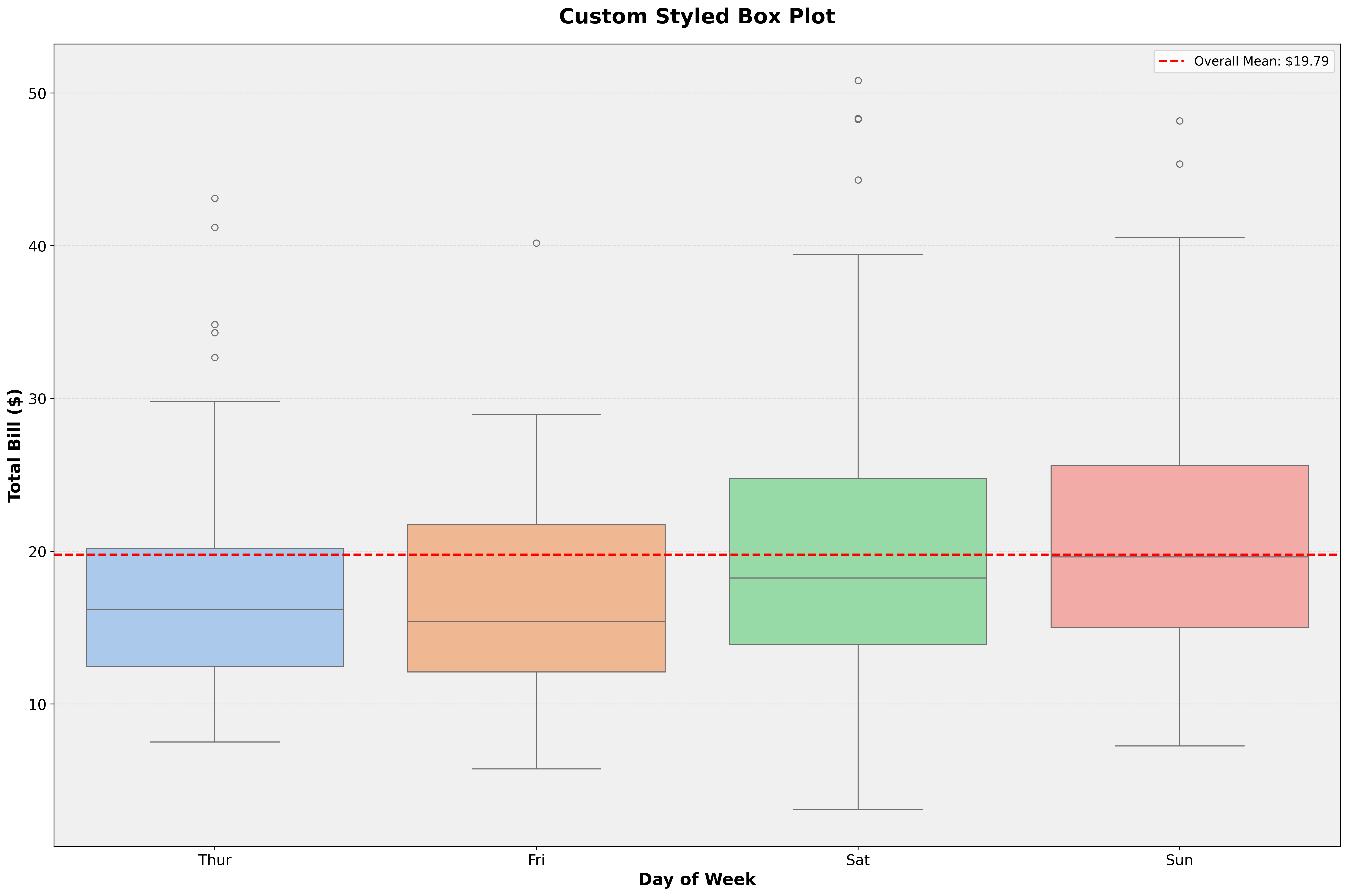
Combine Seaborn with Matplotlib:

fig, ax = plt.subplots(figsize=(18, 12))

tips = sns.load_dataset('tips')

# Create Seaborn plot
sns.boxplot(data=tips,
            x='day',
            y='total_bill',
            palette='pastel',
            ax=ax)

# Customize with Matplotlib
ax.set_xlabel('Day of Week', fontsize=16, fontweight='bold')
ax.set_ylabel('Total Bill ($)', fontsize=16, fontweight='bold')
ax.set_title('Custom Styled Box Plot', fontsize=20, fontweight='bold', pad=20)
ax.tick_params(labelsize=14)
ax.grid(axis='y', alpha=0.3, linestyle='--')
ax.set_facecolor('#f0f0f0')

# Add reference line
mean_bill = tips['total_bill'].mean()
ax.axhline(mean_bill, color='red', linestyle='--', linewidth=2, 
           label=f'Overall Mean: ${mean_bill:.2f}')
ax.legend(fontsize=12)

plt.tight_layout()
plt.show()

Seaborn handles the plot, Matplotlib handles the polish.

Context Settings

Adjust plots for different media:

import matplotlib.pyplot as plt
import seaborn as sns

tips = sns.load_dataset('tips')
contexts = ['paper', 'notebook', 'talk', 'poster']

for context in contexts:
    sns.set_context(context)
    
    fig, ax = plt.subplots(figsize=(8, 6))
    
    sns.scatterplot(
        data=tips,
        x='total_bill',
        y='tip',
        alpha=0.6,
        ax=ax
    )
    
    ax.set_title(f'Context: {context}', fontsize=18)
    ax.set_xlabel('Total Bill ($)')
    ax.set_ylabel('Tip ($)')
    
    plt.tight_layout()
    plt.show()

# Reset to default
sns.set_context('notebook')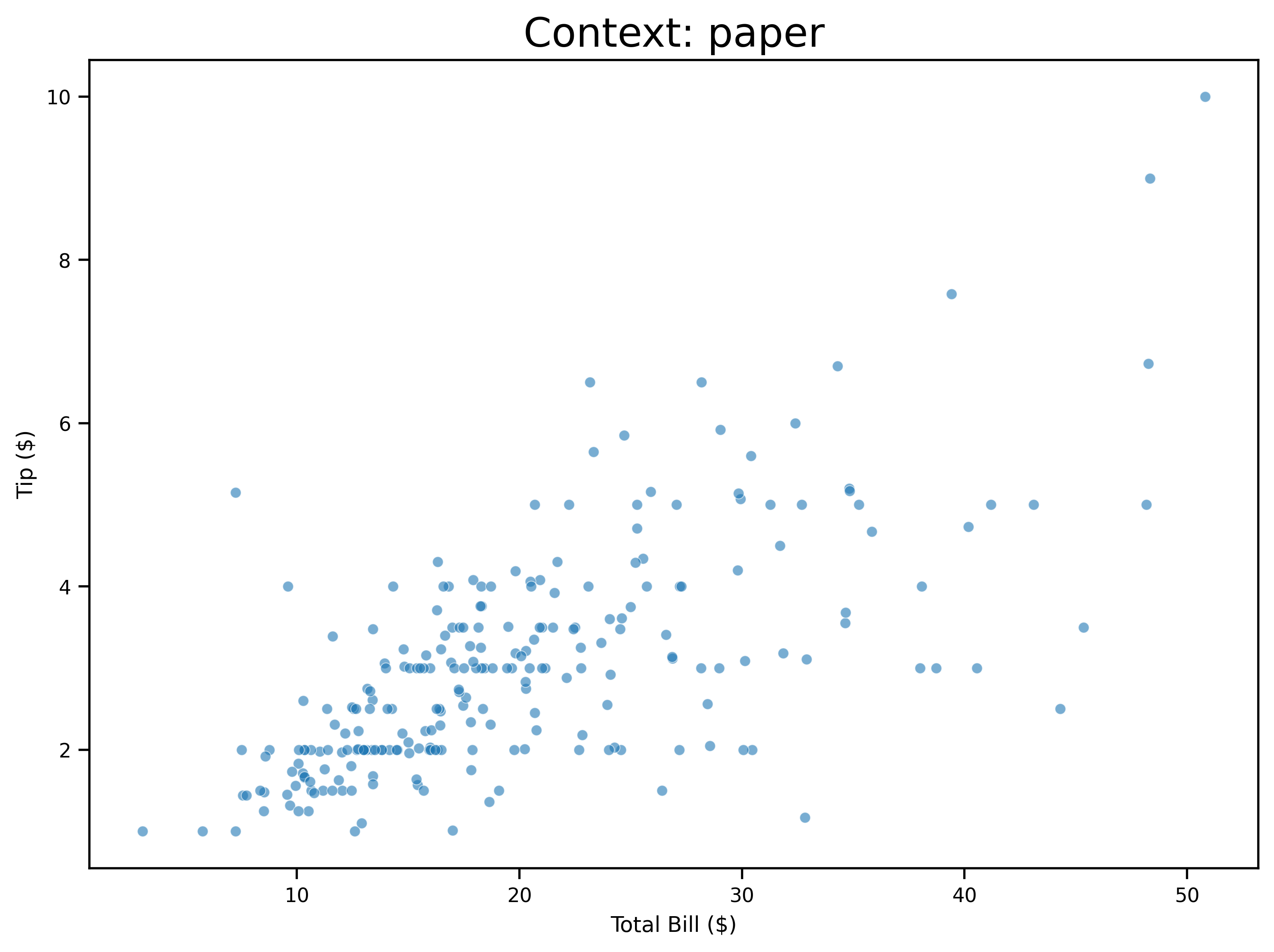

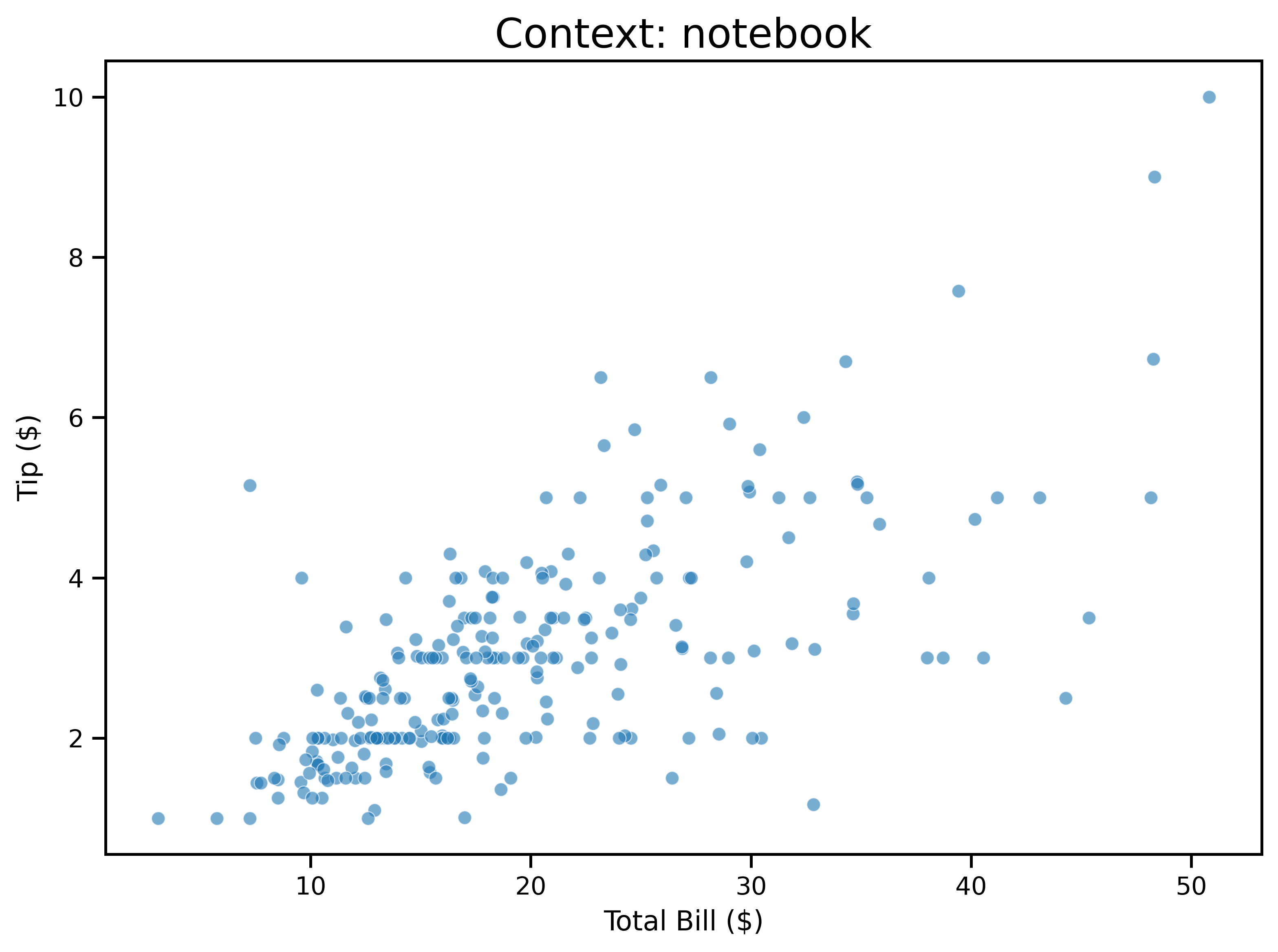
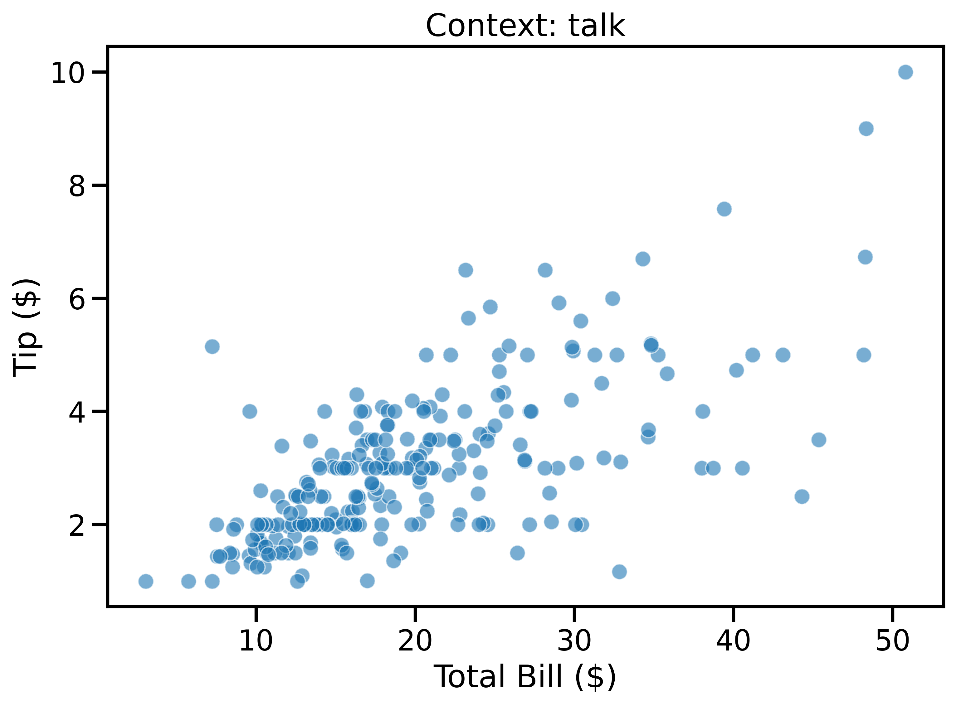
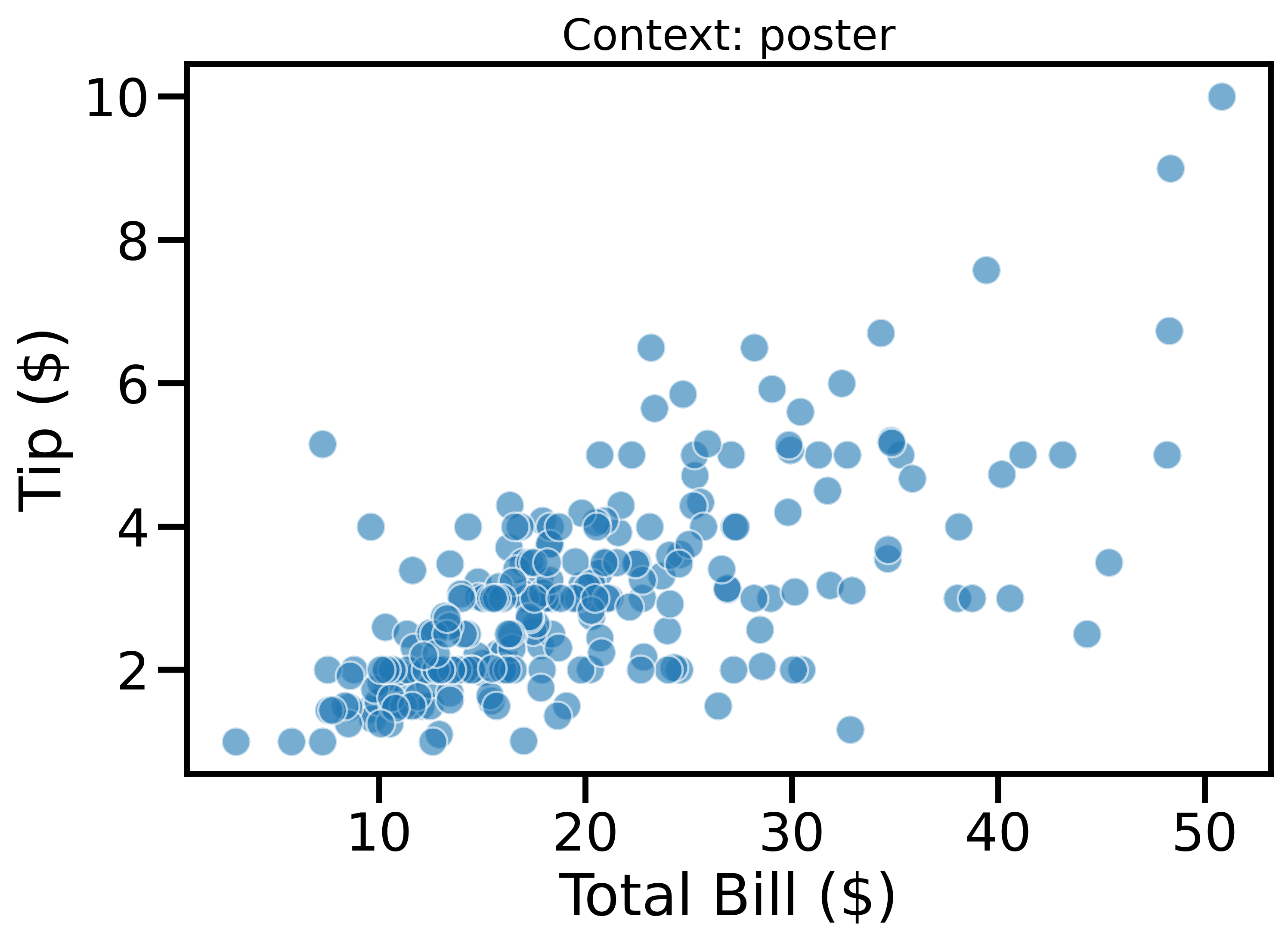
Contexts automatically scale plot elements for different presentation settings.

Time Series with Seaborn

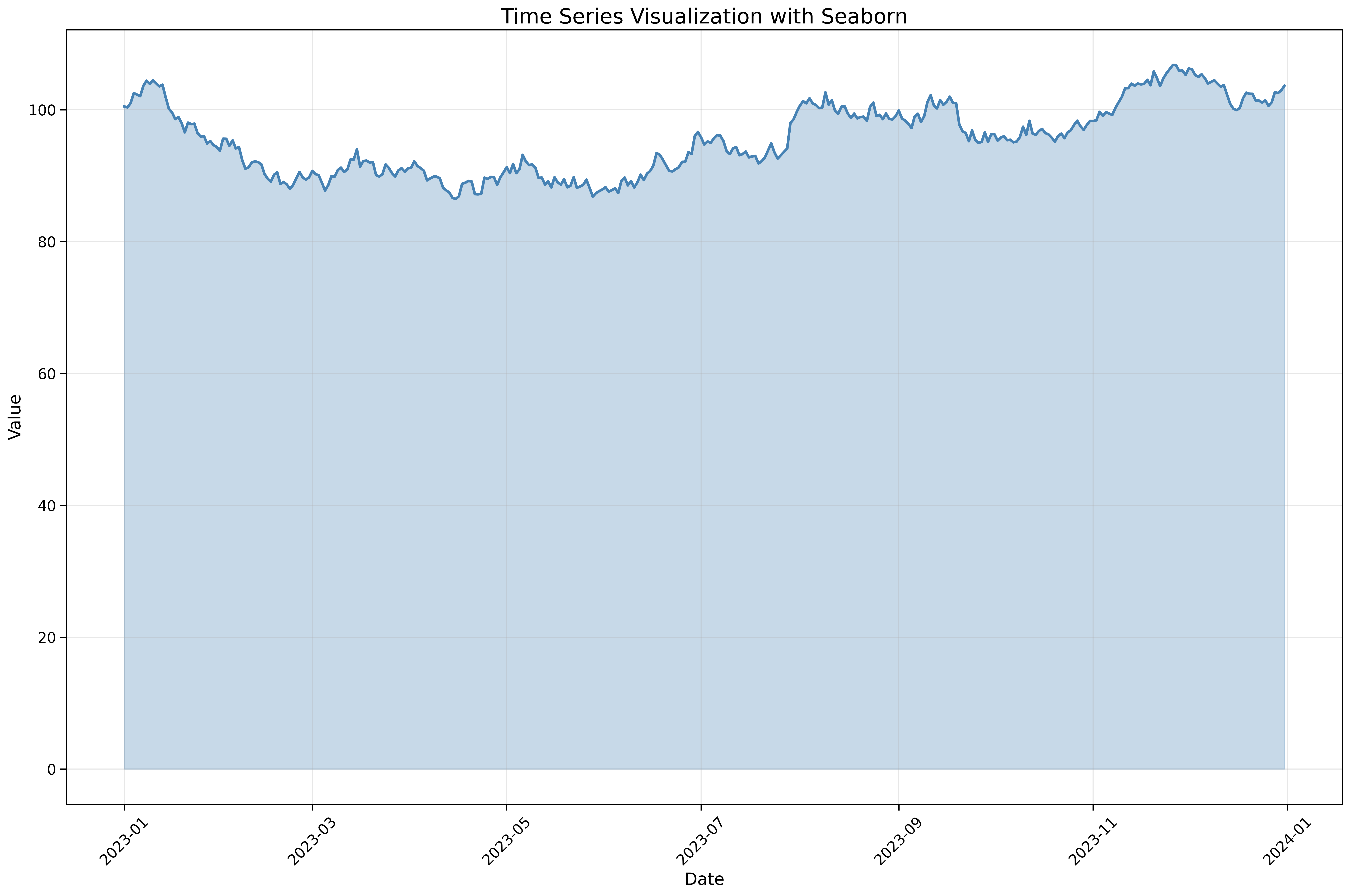
Visualize temporal patterns:

fig, ax = plt.subplots(figsize=(18, 12))

# Create sample time series data
dates = pd.date_range('2023-01-01', periods=365, freq='D')
np.random.seed(42)
values = np.cumsum(np.random.randn(365)) + 100

df = pd.DataFrame({'date': dates, 'value': values})

sns.lineplot(data=df,
             x='date',
             y='value',
             linewidth=2.5,
             color='steelblue',
             ax=ax)

ax.fill_between(df['date'], df['value'], alpha=0.3, color='steelblue')

ax.set_xlabel('Date', fontsize=16)
ax.set_ylabel('Value', fontsize=16)
ax.set_title('Time Series Visualization with Seaborn', fontsize=20)
ax.tick_params(labelsize=14)
ax.grid(True, alpha=0.3)
plt.xticks(rotation=45)
plt.tight_layout()
plt.show()

Seaborn works seamlessly with pandas datetime indices.

Statistical Annotations

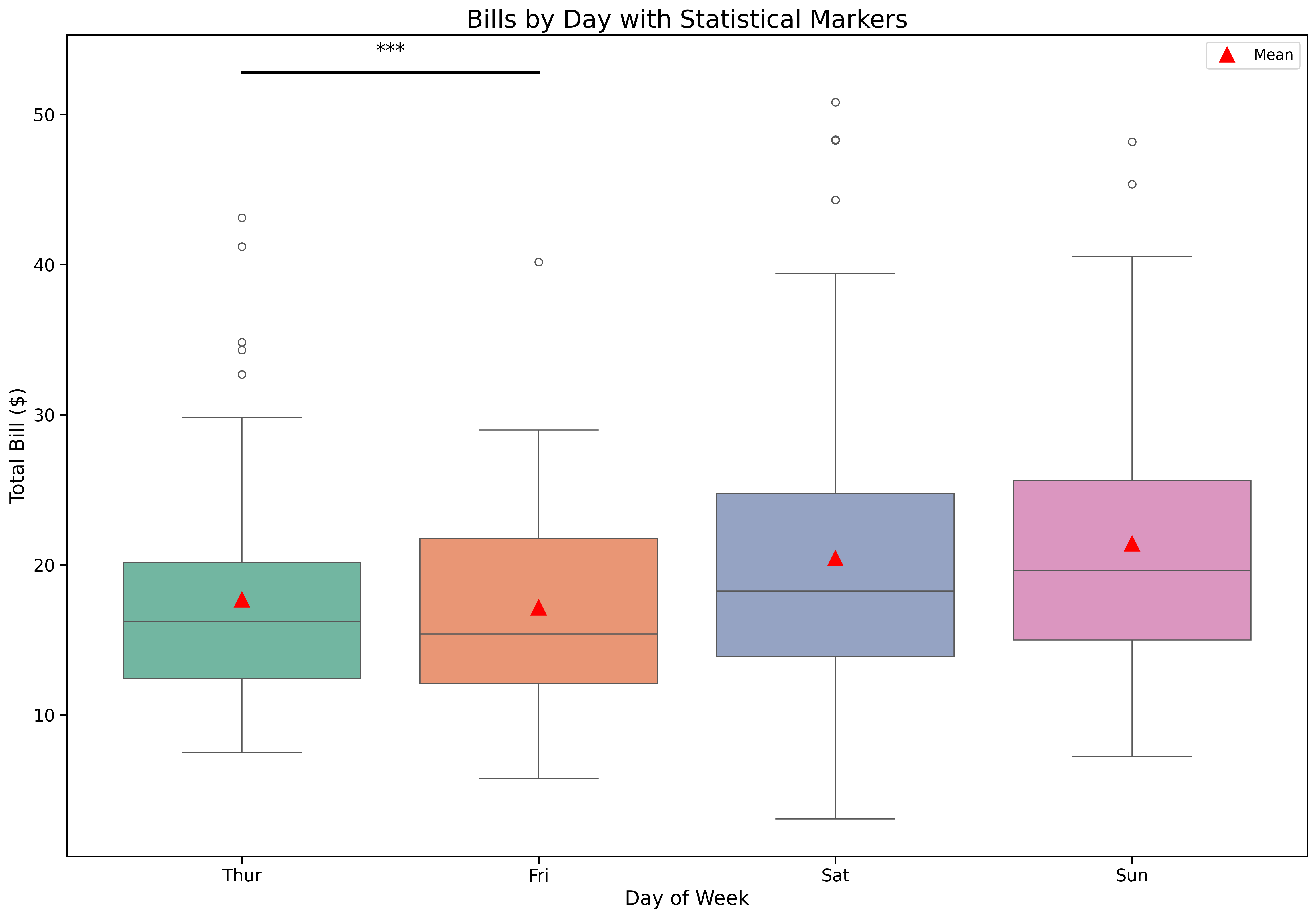
Add statistical test results:

from scipy import stats

fig, ax = plt.subplots(figsize=(18, 12))

tips = sns.load_dataset('tips')

sns.boxplot(data=tips,
            x='day',
            y='total_bill',
            palette='Set2',
            ax=ax)

# Add mean markers
means = tips.groupby('day')['total_bill'].mean()
positions = range(len(means))
ax.plot(positions, means, 'r^', markersize=12, label='Mean', zorder=3)

ax.set_xlabel('Day of Week', fontsize=16)
ax.set_ylabel('Total Bill ($)', fontsize=16)
ax.set_title('Bills by Day with Statistical Markers', fontsize=20)
ax.tick_params(labelsize=14)
ax.legend(fontsize=12)

# Add significance brackets (example)
y_max = tips['total_bill'].max()
ax.plot([0, 1], [y_max + 2, y_max + 2], 'k-', linewidth=2)
ax.text(0.5, y_max + 3, '***', ha='center', fontsize=16)

plt.show()

Combine statistical tests with beautiful visualizations.

Best Practices

Essential Guidelines

1. Choose the right plot type - Match visualization to your data structure
2. Use hue, size, and style - Add dimensions without cluttering
3. Leverage built-in themes - Professional appearance instantly
4. Combine with Matplotlib - Fine-tune when needed
5. Use categorical functions - catplot, relplot, displot for faceting
6. Add context - Titles, labels, and legends are crucial
7. Consider colorblind palettes - Use palette='colorblind'
8. Test with real data - Sample datasets are for learning

Seaborn vs Matplotlib: When to Use What

Use Seaborn When	Use Matplotlib When
Working with DataFrames	Working with arrays
Statistical visualization	Custom/complex plots
Quick exploration	Precise control needed
Multiple categories	Single variable plots
Want beautiful defaults	Need specific styling

Note

Remember: They work together! Use Seaborn for the plot, Matplotlib for customization.

Quick Reference

Plot Type	Function	Best For
Scatter	scatterplot()	Relationships
Line	lineplot()	Trends, time series
Bar	barplot()	Category means
Box	boxplot()	Distribution quartiles
Violin	violinplot()	Distribution density
Histogram	histplot()	Single variable distribution
KDE	kdeplot()	Smooth distributions
Heatmap	heatmap()	Matrices, correlations
Pair	pairplot()	All pairwise relationships
Joint	jointplot()	Bivariate + marginals
Regression	regplot(), lmplot()	Linear relationships

Advanced Resources

Official Documentation: - https://seaborn.pydata.org/

Tutorials: - Seaborn Gallery: https://seaborn.pydata.org/examples/index.html - Matplotlib Gallery: https://matplotlib.org/stable/gallery/

Color Palettes: - ColorBrewer: https://colorbrewer2.org/ - Seaborn Palettes: https://seaborn.pydata.org/tutorial/color_palettes.html

Thank You!

Questions?

Happy Plotting! 🎨📊